Lab 1

Before you begin:

Go to Titanium. Look under the Lab Assignments block. Save the GSS Dataset2.sav to either your desktop or a flash drive (somewhere where you will have access to it throughout the semester). This is the General Social Survey. There is also a GSS codebook available in the same area of Titanium. This shows you the entire text of each question asked by the GSS. It is recommended that you save a copy of this for your reference too.

Ok, now we’re ready to start!

Opening and Examining the Data

1. Open SPSS (either from a computer in one of the campus labs or from home via the Virtual Computer Lab (VCL) or using SPSS software available for free to all students – see links on Titanium) by going to the Start button and going to all programs. Select IBM SPSS Statistics 23 (or an older version of SPSS if that is what is available). Once you have opened SPSS, open the GSS Dataset2.sav that you saved from Titanium. Now that the file is open, there will be an output file that will also open (this always happens when opening data in SPSS). The output is where all of your analysis will be displayed.

2. Now that the dataset is open (there will be [DataSet1] in the top bar), you will notice that there are two tabs at the bottom left of the window: Data View and Variable View. SPSS will open in one of these two windows, just know that you may navigate between the two using this tab. Take a look at the last page of this lab – it explains Variable View.

3. Click on Data View to open the data tab. Notice that there are 170 columns, representing the variables and 2023 rows, representing 2023 respondents or cases.

4. Click on Variable View and peruse the data. If you increase the width of the label column by clicking and dragging its edge, you can see a description of each variable. You can also refer the GSS codebook to see more complete descriptions. Look over all the variables and pick 5 you would like to examine. Two of these variables must be interval in measurement (see Measure column – interval level variables will be listed as “scale”). Pick variables that you think are interrelated.

For example: I’m selecting ‘age’, ‘sex’, ‘tvhours’, ‘R_raceen1’, and ‘visilib’ because I think the number of times one visits the library might vary by, or even be influenced by, one’s sex, race, age, and number of hours spent watching tv each week. (For your Lab, please select variable different than the ones I did – you can have some overlap, put please don’t select the same 5 variables. You may NOT select ‘visilib’ since I use it for all my examples).

Please note that all the variables that start with “ab” measure attitudes towards abortion (not the number of people who have had abortions). For example ‘abrape’ asks people how they feel about abortion in cases of rape. Whereas, ‘abany’ asks people how they feel about abortion for any reason.

5. Complete Question 1 – 2 on the Lab 1 Summary Sheet.

Frequencies Distributions and Charts

Next we want to see how each variable is distributed across the sample. We can do this in 2 ways: by examining the frequency distributions and by creating charts to summarize the data.

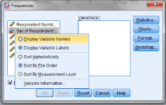
1. At the top of the data file, you will notice typical menu options. To run our descriptive analyses, click on Analyze > Descriptive Statistics > Frequencies. Then select all the variables for which we would like descriptive analyses (select one and move it over to the “Variable(s):” window by clicking the arrow in the middle, or hold CTRL to select multiple variables). To see these variable names, instead of variable labels, right click on one of the names and select Display Variable Names.

*NOTE: Since we’ll be treating data differently depending on its level of measurement, I would encourage you to run separate analyses for each level of measurement for your variables. Consider my example: I have 2 nominal variables (sex and R_raceen1) and 3 interval variables (age, tvhrs, and visilib) so I will run one analysis for the nominal variables and then repeat the process for the interval variables.

2. Next, click Statistics. Under Central Tendency, select mean, median, and mode. Under Dispersion, select range, std deviation, and variance. Then click Continue.

3. Then, click Charts. Select the most appropriate chart for each variable, depending on its level of measurement. Then click Continue.
*NOTE: For my example: I will run the analysis once with my nominal variables. For charts, I can select either pie or bar chart since both work for nominal data. Then I run my analysis again for my interval data, selecting a histogram with normal curve to visually depict the distribution of data.

4. Finally, click OK to run the analysis.

For my example: I will run the analysis once with my nominal variables. For charts, I can select either pie or bar chart since both work for nominal data. Then I run my analysis again for my interval data, selecting a histogram with normal curve to visually depict the distribution of data.

5. Go the Lab 1 Summary Sheet and complete Questions 3 – 4 (see my example below).

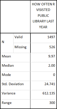
For my example: visilib

I used this table from my output to get all the info I need to complete items 3a – c.

a) List all appropriate measures of central tendency and variability and provide the values.

Mo= 0, Mdn = 2.00, mean = 9.97, R = 300, s² = 612.135, s = 24.741 (Since this is an interval level variable, all measures are appropriate.)

b) Offer Interpretation of at least one of these measures.

Mode: The most commonly occurring answer was 0. More people reported not going to the library at all in the previous year than any other frequency.

c) Is the distribution skewed? If so, which way?

Yes it is positively skewed (I know this because the mean is higher than the median, indicating a few high scores were skewing the distribution).

For item #4:

Variable Type of chart Why appropriate?

Visilib histogram its interval level data

Calculating Confidence Intervals

Now you will calculate Confidence Intervals for your interval variables.

1. Click Analyze > Compare Means > One Sample T-Test. Select all of your interval variables and move them over to the Test Variable(s) window, click on Options to type your confidence interval (95% is default). Click Continue.

2. Click OK.

3. Then repeat the previous two steps but change to 99%.

4. Go to the Lab 1 Summary Sheet and answer Questions 5 – 6 (See my example below).

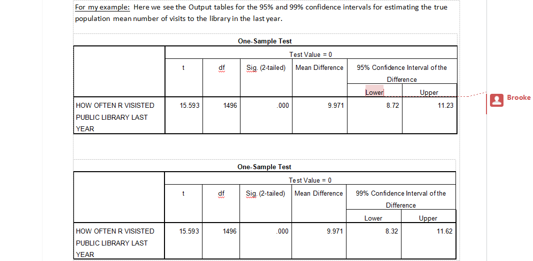
My interpretations would be something along the lines of this:

We can say with 95% confidence that the true population mean number of visits to the library in the last year is between 8.72 and 11.23.

We can say with 99% confidence that the true population mean number of visits to the library in the last year is between 8.32 and 11.62.

To Turn In

You will need submit your lab (including your SPSS Output and your Lab Summary Sheet) online using the submission tool on Titanium. See syllabus for due date. You will be allowed to upload one document for your submission so please be sure to follow the directions below.

You must convert your SPSS Output to a Word doc. Go to your Output file. Click on File > Export. Under Objects to Export, select All. Under Document, Type should be Word/RTF (*.doc). Next, under File Name, click Browse to find a place (like the desktop or your flash drive) where you can place the file. Click Save, then Ok.

Now that you have your SPSS Output saved as a Word doc, you will want to copy and paste the contents of that file into your Lab Summary Sheet file. Now you have one file that contains both your Lab Summary Sheet and your SPSS Output. This is the file you will submit online.