Econ 366-Markets with Frictions Spring 2022
Hello, dear friend, you can consult us at any time if you have any questions, add WeChat: daixieit
Problem Set #1
Econ 366-Markets with Frictions
Spring 2022
Instructions: There are four questions. Each question is worth 25 points. You are encouraged to work in groups of up to 5 members. The problem set is due by midnight of February 16. Please email your solutions to the TA Teresa Steininger at [email protected] . Good Luck!
1. Unemployment BeneÖts in the Moral Hazard Theory of Unemployment. Using the moral hazard model of unemployment of Shapiro and Stiglitz (1984), we want to understand the e§ect on unemployment and welfare of an increase in the generosity of unemployment beneÖts.
a. The equilibrium of the labor market is given by the solution to the following system of equations .

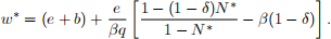
Plot the Labor Demand equation in a graph with N on the horizontal axis and w on the vertical axis. Is the slope of the curve negative or positive? Explain.
b. Plot the No Shirking equation in a graph with N on the horizontal axis and w on the vertical axis. Is the slope of the curve negative or positive? Explain. What happens to the curve as N → 1? Explain..
c. Combining the answer to the questions above, plot both the LD and NS equations. Identify in the graph the equilibrium, and the measure of workers who are unemployed. Since there are workers without a job who are willing to work at the equilibrium wage, why doesnít an individual Örm lower its wage?
d. Using the same type of graph as in part (c), illustrate the e§ect of an increase in the unemployment beneÖt b on the equilibrium employment, wages and unemployment. Interpret your Öndings.
e. Consider the measure of welfare W given by the average utility of an agent in the economy, i.e.

What is the e§ect of an increase in unemployment beneÖts on welfare? Explain your Öndings. Can you think of a di§erent measure of welfare under which the answer may be di§erent?
2. Monitoring technology with false positives. Consider the labor market model of Shapiro and Stiglitz (1984). Suppose that the Örmís monitoring technology returns both false negatives and false positives. SpeciÖcally, the monitoring technology correctly identiÖes a shirking worker with probability q and mistakes him for a diligent worker with probability 1 ━ q , q ∈ (0; 1). Moreover, the monitoring technology correctly identiÖes a diligent worker with probability 1 ━ m, and mistakes him for a shirking worker with probability m, m ∈ (0; q). The Örm Öres all workers identiÖed (correctly or not) as shirkers.
a. Write down an expression for the lifetime utility of a worker employed at the wage w. Explain the meaning of each term in the expression.
b. Derive a condition under which the worker chooses to exert e§ort.
c. Given the monitoring technology described above, the equilibrium employment N* and the equilibrium wage w* satisfy the following labor supply and the no-shirking conditions
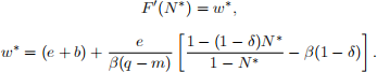
Draw the locus of (w* ; N* ) that satisÖes the labor supply and no-shirking conditions and identify the equilibrium of the economy.
d. What happens to equilibrium wages and employment if the probability m of Öring a diligent worker increases?
e. What happens to equilibrium wages and employment if the probability m of Öring a diligent worker approaches q?
3. Quantifying the e§ect of unemployment beneÖts on unemployment. Consider a version of the labor market model of Pissarides (1985) in which the matching function M (u; v) is uv=(u + v) and the discount factor 8 is 1.
a. Derive an expression for the workerís job-Önding probability, p(7), and for the Örmís job-Ölling probability, q(7).
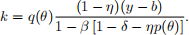
b. Express the equilibrium market tightness 7 in terms of the parameters of the model, k; δ and 6 .
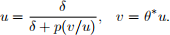
c. Express the equilibrium unemployment u in terms of the parameters of the model.
d. Let y = 1, b = 0:75, δ = 0:025, 6 = 0:5 and k = 0:5. Compute the equilibrium market tightness 7 and the equilibrium unemployment u.
e. If the unemployment beneÖt decreases from b = 0:75 to 0:5, what happens to the equilibrium market tightness 7 and to the equilibrium unemployment u? Explain your Öndings.
4. Vacancy costs and the labor market. Consider the search-theoretic model of the labor market of Diamond (1982), Mortensen (1982) and Pissarides (1985).
a. The equilibrium tightness of the labor market, 7* , solves the following equation
Plot the left and the right hand side of the above equation as functions of 7 and identify 7* .
b. Using the same graph as before, identify the e§ect of an incraese in the vacancy cost k on the equilibrium tightness of the labor market. Interpret your Önding.
c. The equilibrium unemployment, u* , and the equilibrium vacancies, v* , solve simultaneously the following system of equations
Plot the solutions to these two equations in a graph that has u on the horizontal axis and v on the vertical axis (i.e. plot the Beveridge curve and the market tightness curve). Identify u* and v* .
d. Using the same graph as before, illustrate the e§ect of an increase in the vacancy cost k on the equilibrium unemployment and vacancies. Interpret your Öndings.
e. Should the government intervene to lower unemployment in response to an increase in k?
2022-02-16