Hello, dear friend, you can consult us at any time if you have any questions, add WeChat: daixieit

STAT*2050 Statistics II

Winter 2022

Assignment #2

Note: There may be parts of this assignment that will not be graded, but it is in your best interests to do all questions. Notably, your solutions to question 4 will not be handed in, but some answers will be provided. The graded components will be submitted via Crowdmark; you will receive a template for submitting your answers in your email. Further instructions on Crowdmark as well as various hints for completing this assignment will be forthcoming.

1. Refer to the Galapagos data set you analyzed on Assignment #1, question 2. You will use the same data set to answer the following questions.

(a) Obtain the ANOVA table when you conduct a multiple regression analysis with five predictor variables (Area, Elevation, NearestIsland, SantaCruz, AreaAdjacent) and NativeSpp as the response variable. You will need to take logs (use base 10) for all variables; avoid grief from the value of 0 for the distance from Santa Cruz to Santa Cruz by replacing this value with 0.1. What is the value of the multiple R2 when all five predictor variables are included in the model? How does this compare to the coefficient of determination when only log10 (Area) is used as a predictor variable?

(b) Test the hypothesis that at least one of the additional (log transformed) variables improves the model, given that log10 (Area) is already in the model. Note: State your null and alternative hypotheses clearly in terms of the model parameters, and include key evidence (F test statistic value with associated degrees of freedom, p-value) that allows you to draw your conclusion.

(c) Obtain a correlation matrix and a scatterplot matrix for the six (log transformed) variables. As well as Area, Elevation looks like it might provide useful information for predicting the number of native species. Does it do so? (Answer this carefully.)

2. Hand et al. provided the following classic data set from an experiment that measured the absorption over time by potato slices for two types of ions, rubidium and bromide.

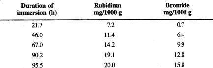
The data is available on CourseLink.

(a) Specify a model equation and state a null hypothesis (in terms of the model parameters) that would allow us to test for nonparallelism of straight lines for the two types of ions. Note: You will need to define an indicator variable; use a (0, 1) coding with rubinium as the base (that is, the value of the indicator variable will be 0 for rubinium, 1 for bromide). You will also need to define an appropriate interaction variable. Use an appropriate ANOVA F-test to test the null hypothesis.

(b) What would the null and alternative hypotheses be in terms of model parameters, if we wished to test for the coincidence of population regression lines in (a)? Conduct the appropriate ANOVA F-test and draw appropriate conclusions.

(c) What would be the value of the F test statistic and associated p-value for testing the null hypothesis that the two lines have the same intercept, if a model without the interaction term was fit? Conduct the appropriate ANOVA F-test and draw appropriate conclusions.

(d) If a SLR (simple linear regression) model was fit to the subset of bromide data, what would be the estimated simple linear regression equation? Show how this can be obtained from the multiple linear regression equation you obtain in (a).

(e) Create two graphs on one page (either side-by-side or top-bottom), with one fitting the model of part (a) and the other fitting the model of part (b). Be sure to label your graphs appropriately.

3. Sokal and Rohlf (1995; Table 16.4; unpublished data of R. K. Kuehn) presented a data set where the response variable Y, the angular transformed frequency of the Lap94 allele in the mollusc Mytilus edulis is to be modelled using polynomial regression as a function of X, the distance off the coast in miles east of Southport, Connecticut. [The angular transformation used was Y (for analysis) = Arcsin[(Frequency of allele Lap94)1/2].

(a) Obtain polynomial models from linear up to and including order 5. Use raw polynomials, not orthogonal polynomials.

(b) Obtain one graph with the estimated linear, quadratic, and cubic model equations of (a) fit to the data. Label appropriately and include a legend. This will be handed in.

(c) Test the null hypothesis that the order 4 and order 5 terms do not contribute to the model (given that terms up to order 3 are already in the model) at the 5% level of significance.

(d) Is it better to use a cubic model than a quadratic model? How do you know this?

(e) Show how the estimated cubic regression equation obtained in (a) can be used to calculated the predicted value of Y and the residual for the first observation in the data set.

4. The Ph.D. thesis of E.G. Kerslake, who completed his Doctor of Veterinary Science degree in 1937, presented a wealth of data on the blood of horses. One data set has been extracted from this thesis and is posted in both Excel and csv file formats. The Excel Workbook format preserves the precision of the decimal places correctly but the csv format (which drops “trailing zeroes”) is easier to read into R. The names on the files start with “Horse Blood, 1937, Table 20". The entire thesis (available as a “historical thesis” through the University of Guelph Library’s Atrium) is also posted so you can see the table as originally presented, and of course your curiosity may compel you to delve further into the thesis. Note that “Horse” is an ID variable while the other five variables are quantitative variables. Of the quantitative variables, Fragility is missing for several horses. An initial challenge here is to subset the data properly in order to make the required analyses.

(a) For the four quantitative variables without missing values, obtain the correlation matrix.

(b) Obtain a “matrix plot” for the variables in (a).

(c) Briefly interpret what (a) and (b) tell us.

(d) Is there a statistically significant correlation between Color.Index and Hemoglobin at the 5% level? In addition to your conclusion, state the null and alternative hypotheses and the evidence (value of test statistic and p-value) you used to draw your conclusion.

(e) What pair of the variables in (a) has the smallest p-value for testing the null hypothesis that the population correlation coefficient is equal to 0 against a two-sided alternative? Report this p-value.

(f) Plot Erythrocyte.mil on Hemoglobin (read this as “Y on X”, that is we will treat Erythrocyte.mil as the response variable and Hemoglobin as the predictor variable in this question). Superimpose the simple linear regression line.

(g) Obtain (individual) 95% confidence intervals for the slope and intercept parameters for the model equation estimated in (f).

(h) Which horse had the largest residual (in absolute value) for the model fit in (f)? What is the value of this residual?

(i) Treating Erythrocyte.mil as the response variable, first fit a multiple regression model with the predictor variables Hemoglobin, Cell.Volume, and Color.Index. Based on a backward elimination procedure, can any variable(s) be removed from the model? If necessary, fit any other models that allow you to arrive at a “best” model for predicting Erythrocyte.mil. What would you recommend as a “best” model based on your analyses? Briefly summarize the evidence (F and/or t test statistics and associated p-values) that you use to make your conclusions.

(j) What is the estimated regression equation for the “best” model selected in (i)? What is the value of the residual for the first horse (#444) in the data set?