Hello, dear friend, you can consult us at any time if you have any questions, add WeChat: daixieit

Due: Tuesday, February 24 at 10:00 AM EDT

Instructions

Your assignment must be submitted by the due date indicated at the top of this document. Deadlines are firm, and the late submission penalty described in the course syllabus will apply starting at 10:01 a.m. on February 24.

Submit your solutions as one PDF file per part of each question on Crowdmark by the deadline. Submissions that combine multiple parts into a single PDF may not be graded. The instructor will not make accommodations for incorrectly uploaded files.

For questions requiring mathematical derivations, handwritten solutions are acceptable only if the uploaded images are clear and neatly organized.

For computational or descriptive questions, all relevant R code must be included in your submission. Failure to provide code when it is used will result in a score of zero for that question.

For interpretation questions, responses must be typed. Text written as comments inside code chunks will not be accepted.

Do not include screenshots of R or RStudio in your submission. Copy and paste your R code and output directly into your document. To include plots, use the Export option in RStudio’s plots window.

Clear organization and professional formatting are part of a complete solution. Marks will be deducted for submissions that are disorganized, difficult to read, or include screenshots of code, output, or plots.

Question 1 [7 marks]

Consider the model (Y ∣ X = x) = f(x) + ϵ, where X and Y are random variables, but X = x is observed, hence fixed. Under this model, we have Var(Y ∣ X = x) = Var(ϵ) = σ 2 . Next, consider a new observation that is not part of the original sample, for which X0 = x0 is observed. The corresponding response Y0 is unobserved and random, and we predict it using ˆ f(x0 ). The error of this prediction problem is:

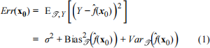
where the expectation is over both the training set T and the new response Y0 , and the bias and variance terms are with respect to the training set T.

a. [3 marks] Suppose W and Z are two random variables, and g is a real-valued function. Show that

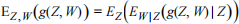
You may assume that all expectations exist.

b. [4 marks] Use the result in part (a) to prove equation (1). This is an alternative (and simpler) proof compared to what we discussed in class.

Question 2 [14 marks]

The data-set Animals from the R package MASS in R includes the average brain and body weights for 28 species of land animals. You may load the data using the following commands:

library(MASS)

data(Animals)

We would like to predict the brain weight using body weight. Once the data is loaded in R , we will study it in the log scale, i.e. log(brain weight) versus log(body weight).

a. [3 marks] Generate a scatter plot of the log body weight on the x axis versus the log brain weight on the y axis. Add to this plot the fitted regression models y = β0 + β1 x + β2 x 2 + ⋯ + βp x p for p = 1, 2, 3, 4, 5, 6. Use different colours for different values of p and include a legend to identify the models. To fit a polynomial regression model of degree q using orthogonal polynomials and you may use the command lm(y poly(x, q)) to do so.

b. [4 marks] Suppose that observations 2, 7, 11, 16, and 26 form the test data set V, and that the remaining observations form the training set T. Fit the polynomial regression model to the training set and use it to predict the responses in the test set. For each polynomial degree p = 1, 2, …, 6, compute the average prediction squared error, APSE, on the test set. Summarize the APSE values for all models in a table and select the best model.

c. [4 marks] Now use five fold cross validation to choose the best degree p = 1, 2, …, 6 for the polynomial regression model. Summarize the cross validation errors for all models in a table and select the best model. For consistency, use the provided indices below to define the five folds in your cross validation.

ShuffledIndices = c(19, 8, 25, 5, 16, 3, 4, 17, 21, 10, 6, 27, 28, 20, 26, 23, 13, 14, 7, 15, 2 4, 2, 22, 9, 11, 18, 12, 1)

folds <- split(ShuffledIndices, rep(c(1, 2, 3, 4, 5), times = c(6, 6, 6, 5, 5)))

folds

## $`1`

## [1] 19 8 25 5 16 3

##

## $`2`

## [1] 4 17 21 10 6 27

##

## $`3`

## [1] 28 20 26 23 13 14

##

## $`4`

## [1] 7 15 24 2 22

##

## $`5`

## [1] 9 11 18 12 1

d. [3 marks] Compare the results obtained in parts (b) and (c). Do they agree on the choice of the best polynomial degree? If not, explain which result you would trust more and why. Compare the composition of the test set used in part (b) with the folds used in part (c), and comment on how this difference may affect the conclusions.

Question 3 [14 marks]

Considering the presence of influential points, which may be viewed as potential outliers, in the Animals dataset, we use the absolute error loss i.e. L(Y, f(X)) = | Y − f(X) | . This loss function is more robust to outliers than the squared error loss.

a. [2 marks] Suppose E denotes the prediction error, defined as E = Y − f(X). On a single plot, overlay two curves representing the loss functions L(E) = | E | and L(E) = E 2 , each plotted as a function of E over the interval E ∈ ( − 5, 5). Describe what you observe by comparing the two curves. In particular, comment on how prediction errors are penalized when the prediction is close to the true value and when it is far from the true value under each loss function.

b. [2 marks] Regenerate the scatter plot from part (a) of Question 2. This time, fit the polynomial regression models using the absolute error loss. You may use the lad() function from the L1pack package in R to fit the models. For example, to fit a polynomial regression model of degree p=3 using absolute error loss, you may use the command lad(y ~ poly(x, 3)) . On the same plot, overlay the fitted models for degrees p=1,2,3,4,5,6 using different colours, and include a legend to identify the models. Compare this plot to the one from part (a) of Question 2, and comment on what you observe.

c. [3 marks] Repeat part (b) of Question 2, but use an absolute error loss function for both fitting the model and measuring prediction performance. To remain consistent with the loss function used in the fitting process, replace APSE with the average absolute prediction error, APAE, defined as

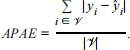
Using this criterion, determine which degree p = 1, 2, …, 6 is selected as the best model. Compare your result with that obtained in part (b) of Question 2 and comment on your findings.

d. [3 marks] Repeat part (c) of Question 2 and select the best polynomial regression model using an absolute error loss function. Use an appropriate R function to fit the models and modify the cross validation error so that it is based on the average of the APAE values across folds rather than the average of the APSE values. Identify which model is selected as the best. State whether this result matches the cross validation result obtained in part (c) of Question 2. Comment on whether you believe this is a fair comparison.

e. [4 marks] Repeat the cross validation calculations twice, once using the absolute error loss and once using the squared error loss to fit the models. In both cases, use the following loss function to measure prediction performance,

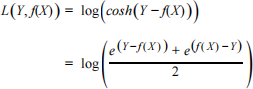
For each fitting approach, compute the cross validation error for all polynomial degrees p = 1, 2, …, 6.

Present the results in a table and select the best model.

Question 4 [10 marks]

Here we will use the final model for prediction.

a. [3 marks] Fit your final model chosen in part (e) of Question 3 to the entire Animals dataset. Generate a scatter plot of the log body weight versus the log brain weight, and overlay on this plot your chosen model.

b. [3 marks] Use the model from part (a) to predict the brain weight for new animals with body weights of 15, 150, 1,000, 5,000, and 12,000 kg. No prediction interval is required.

c. [4 marks] Are each of the predictions in part (b) examples of interpolation or extrapolation? Justify your answer.