DDA5001 · Homework 1
Hello, dear friend, you can consult us at any time if you have any questions, add WeChat: daixieit
DDA5001 · Homework 1
Due: 23:59, Sep 28.
Instructions:
• Homework problems must be clearly answered to receive full credit. Complete sentences that establish a clear logical progress are highly recommended.
• Submit your answer paper in Blackboard. Please upload a file or a zip file. The file name should be in the format last name-first name-hw1.
• The homework must be written in English.
• Late submission will not be graded.
• Each student must not copy homework solutions from another student or from any other source. You are encouraged to discuss with others. However, you must write down the answer using your understanding (after discussion) and words.
Problem 1 (12 points). Concepts and Fundamental Knowledge
(a) (4 points) Concisely state the difference between supervised learning and unsupervised learning.
(b) (4 points) Which one of the following statements is true?
1) Regression is used to fit categorical labels.
2) Least squares must have infinitely many solutions if the number of data points is smaller than feature dimension.
3) The perceptron always converges to a unique linear classifier for a given training dataset.
4) Least squares is a maximum likelihood estimator.
(c) (4 points) Let the data matrix X ∈ Rn×d be a full column rank matrix. Explain why X TX is positive definite (PD). (Hint: Use the definition of linear independence)
Since a PD matrix must be invertible as well, this clarifies why we can take matrix inverse to obtain the unique solution of least squares in case I (where X has full column rank). From an optimization perspective, this PD property also reveals that the least squares in case I is strongly convex.
Problem 2 (17 points). Least Squares Without Full Column Rank
Consider the least squares problem
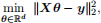
where X ∈ Rn×d , θ ∈ Rd , y ∈ Rn.
(a) (8 points) When n < d, the problem yields infinite many solutions. Assume that rank(X) = n, derive the expression of the infinitely many solutions based on singular value decomposition (SVD). In addition, what is the optimal function value?
Note that the SVD is a notion from linear algebra, and the SVD of the matrix X can be written as
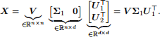
where V ∈ Rn×n is an orthogonal matrix such that VTV = V VT = I, Σ1 ∈ Rn×n is a diagonal matrix taking the form
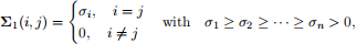
with
σ1 ≥ σ2 ≥ · · · ≥ σn > 0,
U 1(T) ∈ Rn×d is an semi-orthogonal matrix satisfying U 1(T)U 1 = I (but U 1U1(T) ![]() I), and U 2(T) ∈ R(d−n)×d is an semi-orthogonal matrix satisfying U 2(T)U2 = I (but U2U2(T)
I), and U 2(T) ∈ R(d−n)×d is an semi-orthogonal matrix satisfying U 2(T)U2 = I (but U2U2(T) ![]() I).
I).
(Hint: Let A := V Σ1 which is square matrix of full rank, z = U 1(T)θ, solve minz ⅡAz — yⅡ2(2)first, then solve U 1(T)θ = z by considering that U 1(T)U2 = 0.)
(b) (5 points) Later in the overfitting section, we will study that we can also add a regularizer to solve the issue of infinitely many solutions, resulting in the following problem:
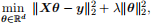
where λ is a positive constant. Derive the unique solution of this problem.
Problem 3 (21 points). Robust Linear Regression
Suppose we have the generative linear regression model y = Xθ⋆ + ϵ ,
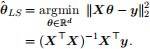
where ϵ is the error term and ϵ ∼i.i.d. N(0, Σ) and X ∈ Rn×d has full column rank. Under this Gaussian noise setup, the maximum likelihood estimator for θ⋆ is given by the least squares:
(a) (6 points) Suppose the error term, ϵ = [ε1,ε2 , ··· ,εn] follows the Laplace distribution, i.e., εi i.![]() .d L(0, b), i = 1, 2, ··· , n and the probability density function is p for some b > 0. Under the maximum likelihood estimation principle, derive the machine learning problem formulation for estimating θ⋆ .
.d L(0, b), i = 1, 2, ··· , n and the probability density function is p for some b > 0. Under the maximum likelihood estimation principle, derive the machine learning problem formulation for estimating θ⋆ .
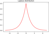
Figure 1: PDF of Laplace distribution
(b) (5 points) Huber-smoothing. ℓ1-norm minimization
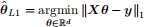
is a popular approach for robust linear regression. However, it is nondifferentiable. We utilize smoothing technique for approximately solving the ℓ 1-norm minimization problem. Huber function is often the choice for smoothing ℓ1 function. The definition and sketch map are shown as below. For some µ > 0,
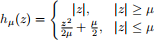
Then,
By using Huber smoothing, the approximation of the above ℓ 1-norm-based robust linear re- gression problem can be smoothed as
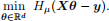
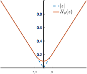
Figure 2: Huber smoothing
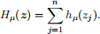
Define
L(θ) = Hµ(Xθ — y),
find the gradient ∇L(θ).
(c) (10 points) Gradient descent for minimizing L(θ). The procedure of the gradient descent method is shown in the following algorithm pseudocode. (We will study the details of the gradient-based optimization algorithms later)
|
1. |
Input: Training data X ,y and initialization θ 0 Huber smoothing parameter µ , total iteration number T, learning rate α . |
|
2. |
for k = 0, 1, ··· , T,do |
|
3. |
θ k+1 = θ k — α∇L(θ k) |
|
4. |
end for |
|
5. |
return θT |
The data set is generated by the linear model
y = Xθ⋆ + ϵ1 + ϵ2 ,
where each entry of ϵ1 ∈ Rn follows i.i.d. Gaussian distribution, while ϵ 2 ∈ Rn is a sparse vector that contains outliers. Given the observed traiing data X and y ,
(1) calculate the estimation θ(ˆ)LS returned by least squares and compute ,,θ(ˆ)LS — θ⋆ ,, ., ,2
(2) suppose n = 1000, d = 50, use Python to implement the gradient descent method to minimize L(θ) in part (b), the parameters are set as µ = 10-5,α = 0.001, T = 1000, plot the error ∥θ k — θ⋆ ∥2 as a function of iteration number. You can download the data {X , y , θ⋆ } on Blackboard.
Problem 4 (24 points). Convergence of The Perceptron for Linearly Separable Data
In lecture, we studied that one iteration of perceptron algorithm will move forward to the currently wrongly classified data. Though such an observation does provide some intuition that perceptron will eventually converge to a linear classifier that correctly separate all the (linearly separable) training data, it is not rigorously justified.
Let us first review the algorithm. The perceptron applies to the linear model
fθ(x) = θ Tx.
At k-the iteration, the algorithm has parameter θ k-1 . Based on θ k-1, the algorithm first pick a wrongly classified data point (xk-1, yk-1) from all the data points ((x1, y1), . . . , (xi, yi), . . . , (xn, yn)), i.e.,
sign (θ k(T)-1xk-1) ≠yk-1 .
Then, perceptron updates as
θ k = θ k-1 + yk-1xk-1 ∀k = 1, 2, . . . (1)
In this question, you will be guided to show that perceptron will eventually stop, i.e., there exists -
a k such that no wrongly classified data exists after at most k number of iterations, and then the perceptron learning algorithm will automatically terminate; see Fig. 3 for an illustration.
(a) Perceptron at the k-th iteration, not all data are correctly classified
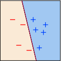
(b) Learned perceptron model after at most k iterations, all data are correctly classified
Figure 3: Illustration of the convergence progress of the perceptron learning algorithm.
Let θ* be corresponding to a classifier that correctly separates all the data points like the one in Fig. 3b. For simplicity, we assume that the initial point of the perceptron algorithm is θ 0 = 0.
The full proof procedure is divided into 5 steps.
(a) (3 points) Let ρ = min1≤i≤nyi(θ*T xi). Show that ρ > 0.
(b) (6 points) Show that θ k(T)θ* ≥ θ k(T)-1 θ* + ρ, and hence conclude that θ k(T)θ* ≥ kρ .
(Hint: Use the update (1).)
(c) (6 points) Show that ∥θ k∥2 ≤ ∥θ k-1∥2 + ∥xk-1∥2 .
(Hint: Use the fact that xk-1 is misclassified by θ k-1.)
(d) (3 points) Show that ∥θ k∥2 ≤ kR2, where R = max1≤i≤n∥xi∥ .
(e) (6 points) Using steps 2 and 4, show that

and hence show that the perceptron learning algorithm must stop within at most

number of iterations.
(Hint: Use the fact  Why?)
Why?)
In practice, perceptron will converge often faster than the above bound. However, since we do not know ρ and θ* in advance, we actually cannot determine the number of iterations to convergence, which does pose a problem if we have non-linearly separable data.
Problem 5 (26 points). Pocket Algorithm for Non-Seperable data
In Problem 4, we have shown that the perceptron algorithm will converge for linearly seperable data. However, for non-linearly separable data, the algorithm will never terminate. In fact, the behavior becomes quite unstable and can jump from a good perceptron to a bad one with only one update (as we will see in this problem). Hence, the quality of Erin cannot be guaranteed.
One simple approach to deal with the unstability is to use the pocket algorithm. The algorithm preserves the parameter θ with the best in-sample error during the update, which ensures mono- tonically decreasing in-sample error. The algorithm is summarized below.
|
Pocket Algorithm |
|
|
1. set the pocket weight parameter θ(ˆ) to be θ 0 |
|
|
2. for k = 0, ··· , T, do |
|
|
3. |
pick a wrongly classified sample from dataset as (x k, yk) |
|
4. |
update as θ k+1 = θ k + ykxk |
|
5. |
if Erin(θ k+1) < Erin(θ(ˆ)): |
|
6. |
θ(ˆ) = θ k+1 |
|
7. |
end for |
|
8. |
return θ(ˆ) |
In this problem, we will implement the performance of perceptron and pocket algorithms based on the US Post Office Zip Code Data, which is a dataset of 16 × 16 grayscale images for digits (0-9). The training dataset has 7291 samples and the test dataset has 2007 samples.
We may extract heuristic features to help us do the classification. Let us focus on the binary classification between digits ”1” and ”6”. In this case, the intensity may be a good feature: the digit ”6” usually occupies larger area than digit ”1”. The asymmetry is another useful feature, as ”1” tends to be more symmetric than ”6”. We can define the asymmetry feature as the average absolute difference between an image and its flipped version.
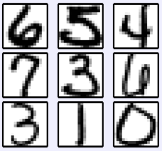
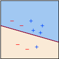
(a) Sample digit images.
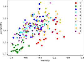
(b) Feature plot of different classes.
Figure 4: Illustration of sample digits and corresponding feature distribution.
1. (10 points) Consider the binary classification problem for digits ”1” and ”6”. Implement the perceptron algorithm and pocket algorithm. The suggested hyperparameters are: threshold = 1e-4, total iteration = 2000, initial parameter θ 0 = 0. (You may implement the algorithms based on the provided source code, where you should finish the part marked as #TODO)
2. (8 points) Plot the in-sample error and the out-of-sample error of these two algorithms versus the number of iterations (for this problem, we consider the training error as the in-sample error, and the test error as out-of-sample error). Note that for the pocket algorithm, the errors are calculated with respect to θ(ˆ) (instead of θ k). Briefly discuss the results.
3. (8 points) Plot 500 data points from class ”1” and ”6”, respectively (similar to the Fig. 4b but with only 2 classes). On this figure, plot the final classification boundary of the two algorithms.
2025-09-26