Q 1.      n = 7 female runners were randomly selected among the first 50 female finishers

of the London Marathon.  The following weights (kilograms) of these runners were recorded before and after the London Marathon:

(a)  Calculate the sample mean and median of the differences of the weights before and after the London Marathon.

 [6 marks]

(b)  Calculate the range, interquartile range, and sample variance of the differ- ences of the weights before and after the London Marathon.

[8 marks]

(c)  Calculate the sample covariance and correlation of the weights before and after the London Marathon.

[8 marks]

(d) Are these data representative of the weight of female runners of the London Marathon? Explain why.

[3 marks]

Q 2.      Let Ⅹ be a continuous random variable with probability density function

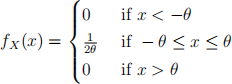
where 0 < θ < o is an unknown parameter.

(a)  Calculate the cumulative distribution function 夕X (α).

[4 marks]

(b)  Calculate the mean and variance of Ⅹ .

[4 marks]

(c)  Calculate the median of Ⅹ .

[3 marks]

(d) Let Ⅹ1  and Ⅹ2  be two independent random variables with probability den- sity function jX . Calculate the probability that Ⅹ1  > 0 and Ⅹ2  < 0.

[4 marks]

(e) Let Ⅹ1．．．．．Ⅹn  be a collection of independent and identically distributed random variables with probability density function jX . Calculate the method of moments estimator of θ .

[10 marks]

[5 marks]

(e) Test the hypothesis

at the 1% significance level, where μ 1  is the mean of the oxygen level for Treatment I and μ2  is the mean of the oxygen level for Treatment II.

[5 marks]

Q 4.      Data have been collected to study the lean body mass in n = 102 male athletes.

The lean body mass (lbm, in kg), weight (wt, in kg), and height (ht, in cm) variables have been imported in R. Sport researchers are interested in under- standing the effect of weight and height on the lean body mass. The following analysis has been carried out in R.

> model1  <-  lm(lbm  ~ wt  + ht  + wt:ht)

>  summary(model1)

#  Call:

#      lm(formula  =  lbm  ~ wt  + ht  + wt:ht)

#

#  Residuals:

#     Min           1Q   Median           3Q         Max

#  -7.9353  -0.7557    0.2131    1.3746    6.9411

#

#  Coefficients:

#     Estimate  Std.  Error  t  value  Pr(>|t|)

#  (Intercept)  -35.386935    29.319616    -1.207    0.23036      # wt                       0.998519     0.347141     2.876    0.00494  ** # ht                       0.279116     0.161547      1.728    0.08718  .  # wt:ht               -0.001570     0.001885    -0.833    0.40706      #  ---

#     Signif.  codes:    0  ***  0.001  **  0.01  *  0.05  .  0.1      1 #

#  Residual  standard  error:  2.256  on  98  degrees  of  freedom # Multiple  R-squared:    0.9495,Adjusted  R-squared:    0.9479 #  F-statistic:  613.7  on  3  and  98  DF,   p-value:  <  2.2e-16

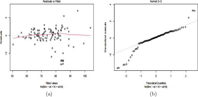
Figure 1: model1 : (a) Residuals vs fitted values plot and (b) QQ-plot.

(a) Write down the mathematical model that has been fitted in model1. What is the estimate of the lean body mass for an athlete with (wt=80 and ht=175)?

State the corresponding assumptions and explain your calculations.

[8 marks]

(b)  Consider the residuals plot for model1 in Figure 1. Explain the interpreta- tion of the plots in Figure 1a and Figure 1b. Do you spot any problem with the model assumptions? If yes, explain which model assumptions might not be reasonable.

[4 marks]

(c) The interaction between weight and height is then removed using the fol- lowing R code:

> model2  <-  lm(lbm  ~ wt  + ht)

>  summary(model2)

#  Call:

#      lm(formula  =  lbm  ~ wt  + ht)

#

#  Residuals:

#     Min           1Q   Median           3Q         Max

#  -8.0842  -0.7282    0.2217    1.4204    6.9818

#

#  Coefficients:

#     Estimate  Std.  Error  t  value  Pr(>|t|)

#  (Intercept)  -11.47816       5.91988    -1.939  0.055359  .    # wt                       0.71018       0.02424    29.301    <  2e-16  *** # ht                       0.14840       0.03805     3.901  0.000175  *** #     ---

#  Signif.  codes:    0  ***  0.001  **  0.01  *  0.05  .  0.1      1 #

#  Residual  standard  error:  2.253  on  99  degrees  of  freedom # Multiple  R-squared:    0.9491,Adjusted  R-squared:    0.9481 #  F-statistic:  923.1  on  2  and  99  DF,   p-value:  <  2.2e-16

Calculate the estimate of the lean body mass for an athlete with (wt=80 and ht=175) and indicate how to calculate a 95% confidence interval using model2  (either a formula or using R commands).   Do the summaries of model1 and model2 suggest an important improvement in the goodness of fit of the model by including the interaction of weight and height?

[6 marks]

(d) Does the analysis support the belief that there is an interaction effect be- tween weight and height for explaining the lean body mass of the athlethes? Carry out the appropriate test of hypothesis at a 0．05 significance level and justify your conclusion.

[7 marks]