Hello, dear friend, you can consult us at any time if you have any questions, add WeChat: daixieit

37902 Foundation of Advanced Quantitative Marketing

Session II (Fall 2024)

Plan of action for the class

- IIA & Elasticity

-  Model fit measures

-  State dependence & Intertia

- Identifying State dependence

1 IIA & Elasticity

• IIA: Independence from irrelevant alternatives

- The ratio of the probabilities of two brands is unaffected by the entry of a new brand that looks a lot like one of them {Pepsi, Sprite} vs {Pepsi, Coke, Sprite}.  In the former case, if the probability of a consumer buying each brand is 0.5, then the ratio of Pepsi to Sprite is  1.   So even after introduction of Coke, the ratio will be preserved according to the logit model.

• Elasticities

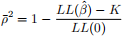
– Own Elasticity=

– Own Elasticity=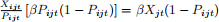

– Cross Elasticity=

– So for all j ≠ k, the cross elasticity will be the same. This is another property of the logit model.

2 Model fit measurement

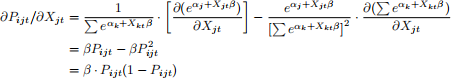
a) The ρ2 - metric

LL(ˆβ) : Value of the log-likelihood at the converged set of parameters.

LL(0) : Likelihood corresponding to no parameters being estimated.

• What is LL(0)?

Suppose there are four choice alternatives with no information about the X variables (feature, display, etc.), the predicted choice probability would be 0.25 for the chosen brand. Then LL(0) = N · ln(0.25) where N is the number of observations in the data.  It can be argued however that we have more information in the choice data than the “chance” assumption of 0.25.  In principle I can compute the share of each of the 4 brands in the data and use them to compute LL(0).   This is equivalent to estimating a logit model only with the intercept or intrinsic brand preference.

•  The ρ2  is loosely interpreted as an R2  type metric although the analogy is not too clear.  It does lie between 0 and 1 though.  Like R-2  there is also a ρ-2  measure that accounts for the number  (K) of estimated parameters,

Note that since LL(·) is negative, ρ-2  < ρ2.

b) The Akaike information criterion

To choose among nested models, a variety of measures exist, the AIC is one of them

AIC = —2L(ˆβ) + 2K

Then pick model with smallest AIC.

c) HQ/BIC/CAIC (Other criteria we did NOT cover in class)

One problem with ρ-2  and AIC is that as the number of observations goes up, one is more likely to pick models with more parameters.  To avoid this over-parameterization, several other criteria have been offered to penalize for number of observations (N).

Hannan - Quinn (HQ) Criterion =—2L(ˆβ) + 2Kln(ln(N))

Bayesian Information Criterion (BIC) =—2L(ˆβ) + Kln(N)

Consistent Akaike Information Criterion (CAIC) =—2L(ˆβ) + K(ln(N) + 1)

Criteria in b) and c) can be used in Nested Hypotheses Testing.

3 State dependence & inertia

One of the fundamental tenets of marketing is engendering loyalty among consumers.  So marketers are in- terested in measuring whether or not their consumers are loyal.  So how to measure the loyalty of a consumer?

One common operationalization of loyalty is by coding up previous brand or previous “state” that the consumer was in when they made a purchase on the last occasion. Hence state dependence is the technical term for a measure of loyalty that we use in marketing.  The most common measure of loyalty is just the previous purchase indicator included as an additional variable in the logit model.

This is also referred to as the “first-order state dependence” model.  Here the “loyalty” of household i for brand j when makeing a purchase at time t can be written as

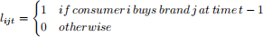
So lijt  is just the lagged version of the choice data that you use to construct the likelihood.  Then the model becomes:

Uijt  = αij  + Xijt βi + lijt δi + ϵijt

where αij  and βi  are defined as

αij  = αj  + Zi (λj  - λJ )

βi  = β + Ziγ

δi  = δ + Zi ν

When lagging the purchase variable to create the loyalty variable, notice you will lose the first observation for each household.  So instead of 2430 data points, you now have only 2330 data points.  You need to be careful when you are comparing this model to the one without the loyalty variable.

Some observations:

1) If the estimated δi  < 0, then this is taken as evidence of “variety-seeking”.

2)  There are several other operationalizations of the loyalty variable.   The  most  common  one  is  the Guadagni-Little (MKSC, 1983) version that is given as follows:

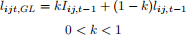
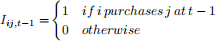
(Recall Iij,t- 1  was the same as lijt  in the first-order state dependence model).  There are 2 issues with using lijt,GL

You will lose a lot of observations when you create the loyalty variable as you need to go further back in history.

To create the lijt,GL  variable you need to know the value of k. Usually researchers perform a “grid search” on k, i.e., they fix k = {0.1, 0.2, 0.3, ..., 0.9} and for each k, calculate lijt,GL  using the first 3-4 purchases of each household.  Then they create the loyalty variable for the remaining purchases and use it in the logit model.  Next they look at the model fit for each value of k and pick k that maximizes the log likelihood. An alternative followed by most researchers is to simply fix k = 0.8.

Problem with including the loyalty variable:

Note that the lagged purchase is simply the lagged dependent variable.  So it is not surprising that in product categories where consumers tend to repurchase the same brand, model fit would improve consider- ably by including this variable.

Problem: A consumer can be loyal because of “true” state dependence (meaning as a marketer you may want to use free samples) or because of strong preference for the brand:  a high αi  (meaning I want to invest in advertising to increase preference). How to separate the two?

The answer to the above question requires us to allow consumers to have different preferences (i.e., αj’s) in a flexible fashion.   This is our next step in the journey.   Before that a note on identification of state dependence. Ideally we want to think of an intervention that “randomly” changes the brand consumers end up buying (e.g., a deep price cut or a stockout).  Now if consumers persist buying this brand that they ended up buying for exogenous reasons. This would be evidence for state dependence.

4 Recent approaches to identifying state dependence (SD) - Hurri- canes, Earthquakes and Stephen Colbert

Hurricanes accelerate purchases among consumers so some consumers who typically buy, say Dasani water, may not be able to find it when they go to shop to stock up for the hurricane.  This will lead to a switch away from Dasani to say, Crystal Geyser.  If there is state dependence, then the consumer will likely continue to buy Crystal Geyser after the hurricane period. If it goes back to Dasani then there is no state dependence. The idea behind the hurricanes paper (Seiler & Levine, MKSC 2023) is to see if purchases “revert” back to pre-hurricane brands even if there was a switch during the hurricane period.  They are interested in short run effects. They find reversion to the previous brands quickly indicating a lack of evidence for state dependence. They also show that imposing a functional form on SD as we did in class may lead to the finding of spurious state dependence.

While the above paper focuses on short run effects, the earthquakes paper (Carlos Noton and co-authors Working paper), focuses on the impact of switching due to longer term absences of a consumer’s favorite brand.  If, say, Dasani was absent for 6 months from myy store, would I switch back when it became  (re- )available?  The finding here is of state dependence - purchases do not revert back after a ong absence and smaller brands benefit from the absence of the bigger brands from the shelves.

Finally the Stepehn Colbert paper (Rishabh, Tuchman & Chintagunta, WP), shows that an exogenous shock that increases the likelihood of a particular state - “Success” - of a donation to a charitable cause, is likely to engender “loyalty” in the sense that the donor is more likely to make a send donation on the platform.