1.  Suppose that the price of a certain good at market equilibrium is £50 and the quantity sold is equal to 20.  At this equilibrium, the price elasticity of supply is 2.  Further assume that the supply curve is linear.

(a)  Using price elasticity and the equilibirum market outcome, find the equation for the supply curve.

(b) At market equilibrium, what is the producer surplus?

(c)  Imagine that a policy results in price falling from £50 to £40. What will be the change in producer surplus?

(d) What fraction of the lost producer surplus is due to the reduction of quantities supplied? What is the driving force behind the remaining loss in producer surplus?

Solution:

(a)  The supply schedule has the following form:

Using elasticity, first find the value of 

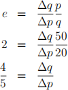
Using linearity and equilibrium outcome (20, 50)

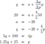
(b)  The producer surplus is the area between the price line (p = 50) and the inverse supply

schedule from q = 0 to q = 20. Note that this area forms a triangle with height equal to price minus the price at q = 0 (which is 50 − 25 = 25) and base equal to the equilibrium quantity 20. Therefore, the producer surplus in this market is £0.5 ∗ 25 ∗ 20 = 250 (see Figure 1).

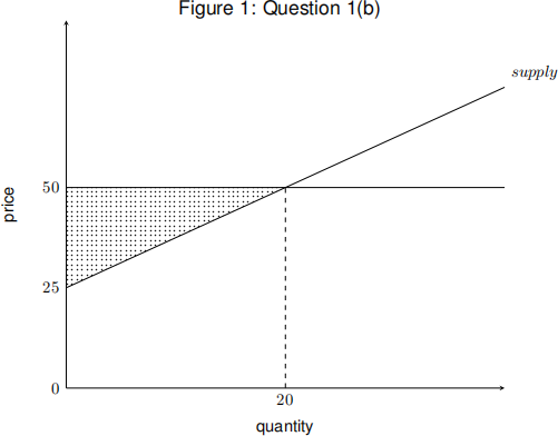
(c)  Using the supply schedule, we see that at price £40, the quantity supplied falls to 12. The loss of producer surplus is equal to the area of the trapezium between the old and new price and the old and new quantities sold (see Figure 2).  The loss of producer surplus is equal to 10 ∗ 12 + 0.5 ∗ 8 ∗ 10 = 160

(d)  The loss ofproducer surplus represented by the trapezium can be divided into a rectan- gle over the quantity still supplied and a triangle over the quantities no longer supplied. The area of this rectangle is 120 and the area of the triangle is 40. Thus, 40 is the loss in producer surplus due to the reduction in the quantity sold and the remaining 120 is due to producers receiving less for each unit that they continue to sell.

(b) Possible limitations

•  Substantial data requirements – requires a large amount of information on product attributes

•  Bundling – implicit assumption that bundles of products vary in all attributes, but this may not be the case in practice

•  Multicollinearity – individual attributes may be strongly related (educated parents and high-income households), making it hard to identify the implicit price of a single attribute

•  Modelling – involves making assumptions about how individual attributes affect price

• Also assuming individuals make decisions on the basis of full information (e.g. are they really fully aware of school quality?)

•  Selection issues - individuals who value school quality will choose to live nearer

Section B

4.  Consider a hypothetical market for cauliflower. At equilibrium, the price for each unit is £2.  At this market clearing price, 1000 cauliflower units are sold.  Farmers are currently not happy with the price for their agricultural produce, so the government is considering implementing a legislation that will put a minimum price cap of £3.  Assume that after the price increase, farmers are willing to sell more units but the demand is only for 900 units. Further assume that the market demand and supply curves are linear and that the market reservation price (the lowest price at which any farmer is willing to sell) is £1

(a) Compute the dollar value of the impact of this policy on farmers, consumers and the society as a whole.

(b)  Because of the increased price, demand in the secondary market for broccoli in-

creases. Assume that the price of broccoli is set equal to the marginal cost and that the marginal costs are constant (i.e. the supply curve is horizontal). Further, assume that there no additional externalities resulting from the reduced use of cauliflower or the increased use of broccoli.  Are there any additional costs or benefits due to the increased demand for broccoli? Explain.

(a)  We know two points on the supply curve (0,1) and (1000,2).  Using this the equation

for supply curve will be

Further, we know two points on the demand curve (900,3) and (1000,2). Using this the equation for demand curve will be

Due to the minimum price legislation, consumers will face a reduction of their consumer

surplus equal to the area of the trapezium: £(3 − 2) ∗ 900 + 0.5 ∗ (3 − 2) ∗ 100 = 950      Farmers have dual impact.  A part of producer surplus is lost due to the reduction in supply. This is equal to the area of the triangle: £0.5 ∗ 100 ∗ 0.1 = 5. For the remaining

quantities still sold in the market, producers’ gain a surplus equal to area of the triangle £1 ∗ 900 = 900. The net effect is an increase of producer surplus equal to £895.

The net effect of this policy is a loss of surplus equal to £55.

No additional costs or benefits result from the outward shift in the demand curve for

broccolis. Although the shift in demand implies that broccoli is now more highly valued, the increase in cauliflower price makes neither current broccoli consumers nor new broccoli consumers better off.  Any effects in the secondary market for broccoli are already fully incorporated into the primary market demand curve of cauliflowers.

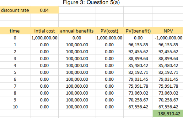
5.  The government of a certain country would like to preserve a piece of its land as a wilderness area. The current land owner offers to lease the land for 10 years in exchange of a lump-sum payment of £1 million to be paid at the beginning of the 10-year period. The government estimates that the land would generate a benefit of £100,000 at the end of each of the 10 years.

(a) Assuming a real discount rate of 4%, calculate the present value of the net benefit of leasing the land.

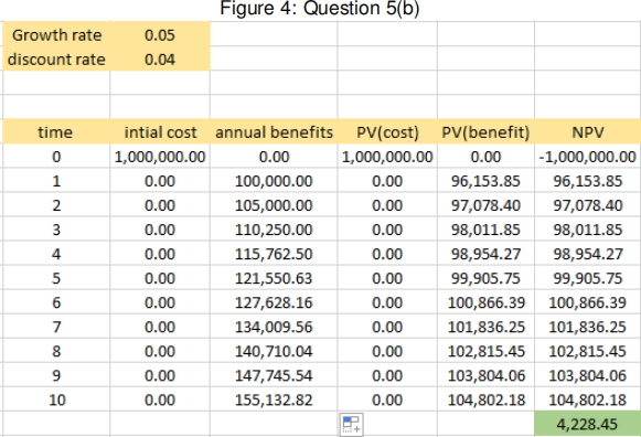
(b) Some analysts estimate that the annual real benefit will actually grow at a rate of 5%.

Recompute the present value of the net benefit assuming that these analysts are cor- rect.

(c)  Imagine that the owner is willing to sell the land for £2 million.  Further, suppose that the annual benefit of the land is assumed to be £100,000 (accruing at the end of each year) and the real discount rate is 4%.  If the government purchases the land as a permanent wildlife area, what will be the net benefit of this purchase?

(a)  Net benefits = £-188,910 (see Figure3)

(b)  Net benefits = £4,228 (see Figure4)

(c)  PV(cost) = £2,000,000

PV(benefits) = 100,000/0.04 = £40,000,000

Net benefits = £500,000

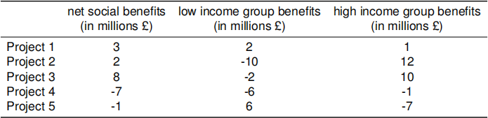
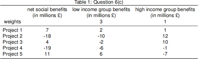
6.  A city is considering five public projects.  Suppose that the city has enough budget to implement all projects that will increase the welfare of its citizens.  Moreover, none of the projects are mutually exclusive.  The local government hires an analyst to analyse the ef- fectiveness of each of the five proposals. The analyst finds that the projects have different benefits for the low-income households and the high-income households. The findings from the CBAs are summarized in the table below.

(a) According to the net benefit rule, which of these projects should be implemented? (b)  For which of these projects might distributional considerations be an issue?

(c)  Recompute the net social benefits for the five projects using a distributional weight of

3 for the low-income group and 1 for the high-income group. Under the weighted-CBA which projects should be implemented?