Hello, dear friend, you can consult us at any time if you have any questions, add WeChat: daixieit

Final project

Computational Finance with Python

General information

Marking and credit

This project contributes 90% towards the final mark for the module. In each exercise, marks are allocated for both for coding (style, clarity and correctness) and accuracy of numerical results, and for explanations and written work (including comments and doc- strings in the code).

The marks indicated are indicative only.

Partial credit will be given for partial completion of an exercise, for example, if you are able to do a Monte Carlo estimate with fewer paths or time steps.

It may prove impossible to examine projects containing code that does not run, or does not allow data to be changed. In such cases a mark of 0 will be recorded. It is therefore essential that all files are tested thoroughly in Colab before being submitted in the VLE.

Academic integrity

You may use and adapt any code submitted by yourself as part of this module, including your own solutions to the exercises. You may use and adapt all Python code provided in the VLE as part of this module, without the need for acknowledgement. Any code not written by yourself must be acknowledged and referenced.

This is an individual project. You must not collaborate with anybody else or use code that has not been provided in the VLE without acknowledgment. This includes, for ex-ample, discussing the questions with other students, actively using discussion forums or using generative artificial intelligence (such as ChatGPT). Please consult the University’s Student guidance on using AI and translation tools and Policy on Acceptable Assistance with Assessment. Collusion and plagiarism detection software will be used to detect academic misconduct, and suspected offences will be investigated.

Submission instructions

Submit your work by uploading it in the VLE by Friday 23 May at 10am. Work should be submitted as follows:

• Code (and numerical results) should be submitted in the form of Colab notebooks. Code will be tested using unseen test data: use variables to store parameters rather than using hard-wired values.

• Written text should be submitted in pdf format. Scans of handwritten text are ac- ceptable, provided that they are legible.

• Use a separate set of files (ipynb and pdf, as appropriate) for parts 1 (Black-Scholes model) and 2 (Local volatility model). “Part1.ipynb” or “part1.pdf” are examples of sensible filenames.

Late submissions will incur a penalty according to the standard rules for late submission of assessed work. It is advisable to allow enough time (at least one hour) to upload your files to avoid possible congestion in the VLE. In the unlikely event of technical problems in the VLE please email your files in a zip archive to [email protected] before the deadline.

1 Black-Scholes model

Consider a risky asset with stock price S that follows geometric Brownian motion below under the risk neutral measure Q, in other words,

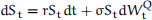
or, equivalently,

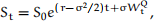
where r is the risk free rate, σ is the volatility and WQ is a standard Brownian motion under Q.

A popular method for approximating the log price is by using the trinomial tree with N steps in which, at each time step n (reflecting the time point n∆t in “real time”), the approximation to the log price ln St evolves as follows:

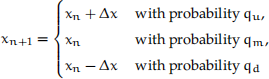
for all n = 0, . . . , N − 1, where ∆x > 0.

1.1 Stock price encoding

At each time step n, the log price xn in the trinomial model takes 2n + 1 different values, with each value being of the form

ln S0 + (ku − kd)∆x,

where ku is the number of “up”jumps and kd the number of “down”jumps, where n − ku  − kd  ≥ 0 is the number of steps in which the price didn’t jump up or down. It is convenient to store all possible log price values in a vector

[ln S0 − n∆x   ln S0 − (n − 1)∆x   ···   ln S0     ln S0 + ∆x   ···   ln S0 + n∆x] .

•  S0  = 59.78.

•  N = 720.

1.3 Vega

Exercise 1.3 (Vega: 10% of project mark). The trinomial method can be used to approximate the value of the vega V = ∂σ/∂V , where V = V(S0, r, σ, T,K) is the value at time 0 of a call option with strike K and maturity date T in the Black-Scholes model with parameters r    and σ .

1. Use a central finite difference approximation to express V in terms of V(S0, r, σ + h, T, K) and V(S0, r, σ − h, T, K), where h > 0.

2. Write a Python function that uses the function you created in Exercise 1.2 to ap-proximate the vega accurately to d decimal places. Your function should take the arguments S0, T, r, σ, N, f and d.

3. Use your function to approximate the vega of a call option with strike K = 62 accu- rately to d = 5 decimal places in a model with the following parameters:

• T = 2.

• r = 0.05.

•  σ = 0.26.

•  S0  = 59.78.

•  N = 720.

2 Local volatility model

A model for a stock S is given by the stochastic differential equation

(1)

where WQ is a Brownian motion under the risk-neutral probability Q. Here r is the risk- free interest rate and S0 is the initial stock price.

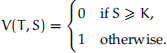
The aim of this part of the project is to use Monte Carlo and finite difference techniques to study a European style derivative where the payoff at time T = 1 is

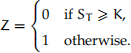
Take K = 96 together with S0  = 96.0 and r = 0.04.

2.1 Finite difference method

The price of the derivative at time t can be expressed as V(t, St), where the function V satisfies the partial differential equation

(2)

for all t ∈ [0, T) and S > 0, with final value

Exercise 2.1 (Forward Euler method: 25% of project mark). Design an explicit (forward   Euler) finite difference scheme to approximate the solution to the partial differential equa- tion in Equation 2. Your work should include the following:

1. Convert the final value problem into an initial value problem.

2. Explain why the boundary conditions

(3)

are appropriate for pricing this derivative.

3. Define a suitable grid to discretize the domain of V, and derive an iterative scheme in matrix form that would allow you to approximate the value of V at the grid points, using the boundary values in Equation 3.

4. Demonstrate numerically using Python that the scheme is unstable for some choices of the step sizes.

5. Write a Python function to implement the iterative scheme. Your function should have suitable arguments and return values. Recall that the parameters of the model were given at the start of the question.

6. Use your function to produce an approximation to V(0, S0).

2.2 Monte Carlo method

Applying the Itô formula to the transformation Xt  = ln St (in other words, St  = eXt) leads to the stochastic differential equation

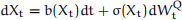(4)

with initial value X0 = ln S0 for the log price process X, where

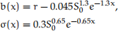
for all x ∈ R.

Exercise 2.2 (Monte Carlo estimate: 30% of project mark). Implement Monte Carlo simu- lation to estimate the price of this derivative at time 0 under Q, as follows.

1. Apply the Lamperti transform in Equation 4 to obtain a diffusion process Y with constant volatility.

2. Write down a statement (step by step) of the Monte Carlo procedure to estimate the price of the derivative by applying the Euler scheme to Y and using antithetic sampling.

3. Implement the procedure in Python. Report the Monte Carlo estimate of the price, the standard error and an approximate 95% confidence interval with 200000 paths and 1000 steps per path.