BCSC/CSC/DSCC 229, DSCC 449: Computer Models of Human Perception and Cognition Homework Assignment #3
Hello, dear friend, you can consult us at any time if you have any questions, add WeChat: daixieit
BCSC/CSC/DSCC 229, DSCC 449: Computer Models of Human Perception and Cognition
Homework Assignment #3
Instructions: Answer all questions below. Include all requested calculations and graphs. Also include the Python code that you wrote to answer the questions. When writing text or equations, please write NEATLY!
(0) (Part A) At the top of the document you turn in, place your name and the date. (Part B) Next, please take the honor pledge. That is, write (by hand using a pen): “I affirm that I have not given or received any unauthorized help on this assignment, and that this work is my own.” Then sign your name.
(1) Implement (using Python) the basic model described in:
Tenenbaum, J. B. & Griffiths, T. L. (2001). Generalization, similarity, and Bayesian infer-ence. Behavioral and Brain Sciences, 24, 629-640.
First, re-read the article (several times) to make sure you understand the model. Given a data set X, the model should produce the probability distribution p(y ∈ C|X) where y is a test point and C is a “consequential” region (e.g., see Figures 1, 2, and 3 of the article). For the sake of simplicity, you can assume:
❼ Individual data points x are integers between 0 and 100.
❼ Individual test items y are integers between 0 and 100.
❼ Individual hypotheses are intervals with integer-valued endpoints (e.g., as illustrated in Figure 1 of the article).
❼ The prior distribution over hypotheses is a uniform distribution (not an Erlang distri-bution).
❼ You’ll need to define hypothesis spaces consisting of hypotheses ranging from a cardi-nality of 1 up to hypotheses with a cardinality of N. For part (a) below, set N = 6.
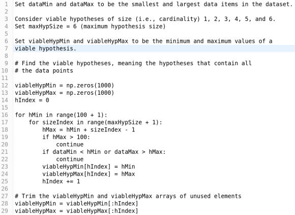
Figure 1: For Question 1, there are many ways to define the viable hypotheses. The method in this figure defines every possible hypothesis, and then determines if a hypothesis is viable or not (a hypothesis is not viable if its maximum value is greater than 100 or if the hypothesis does not contain all data items).
For the remaining parts, set N = 40. [Hint: See Figure 1.]
❼ For each part of this question, produce a graph like the one shown in Figure 2.
(a) Let X = {45}. Plot p(y ∈ C|X) for all y in the interval [38, 52].
(b) Let X = {43, 44, 45}. Plot p(y ∈ C|X) for all y in the interval [0, 100].
(c) Let X = {37, 42, 45}. Plot p(y ∈ C|X) for all y in the interval [0, 100].
(d) Let X = {15, 35, 45}. Plot p(y ∈ C|X) for all y in the interval [0, 100].
(e) Let X = {37, 45}. Plot p(y ∈ C|X) for all y in the interval [0, 100].
(f) Let X = {37, 40, 42, 45}. Plot p(y ∈ C|X) for all y in the interval [0, 100].
(g) Let X = {37, 38, 40, 40, 41, 42, 43, 45} (note that the number 40 occurs twice in this set). Plot p(y ∈ C|X) for all y in the interval [0, 100].
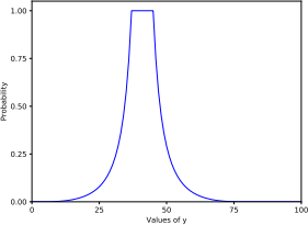
Figure 2: Graph for Question 1(f). Horizontal axis plots test values y. Vertical axis plots p(y ∈ C|X).
(2) (This question is adapted from Problem 10.6 of an early draft of the textbook by Ma, K¨ording, and Goldreich.) You will implement (using Python) the model described in Section 10.3 of the textbook by Ma et al. Please read this section (several times) to make sure you understand it. In particular, you will need to implement Equation 10.35-10.36 (even though there are two equation numbers, there is only one equation).
(a) Implement the model with the goal of generating two figures. The first figure should recreate something like Figure 10.3A from the textbook. (Your figure may look slightly different.) That is, plot the value of d for each set of values for x1 and x2. Let x1 and x2 each vary between -50 and 50. Set σ1 = 3, σ2 = 10, σs = 10, and psame = 0.5. The second figure should be the same except you will plot the decision (same or different) for each set of values for x1 and x2. Thus the plot will be white (same) and black (different).
(b) Repeat part (a) except set σs = 3 (instead of σs = 10 as in part (a)). Does the model now decide “same” more often or decide “different” more often? Why? Please explain the underlying reasons for the difference you see.
(3) The goal of this question is to give you practice with the Metropolis-Hastings (MH) algorithm.
(a) Sample ten data items from a univariate normal distribution with a mean of 10.0 and a variance of 1.0. Next, pretend you don’t know the mean of this distribution. Instead, use the 10 data items to infer a posterior distribution of the mean using the MH algorithm (for now, assume that you know that the data were sampled from a normal distribution with a variance of 1.0). Assume that the prior distribution of the mean is a uniform distribution. Let the proposal distribution be a normal distribution with a standard deviation of 0.05. Initialize your chain to a value of 0.0, and run the chain for 5000 iterations. Create a graph in which the horizontal axis gives the iteration number, and the vertical axis gives the sample value of the chain. [Hint: See Figure 3.]
Hint: Be careful when computing the quantity R. For example, if you compute the likelihood for the proposed value of the mean based on all data items, then this likelihood will go toward zero (because you’ll be multiplying 10 very small numbers). Instead, you’ll need to compute R incrementally, one data item at a time. Using the notation from the lecture slides, let Ri be
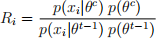
where xi is the i th data item. Then

Computing R in this way is much more robust.
(b) Repeat Part (a) except now use the MH algorithm to estimate both the posterior distri-bution of the mean and the posterior distribution of the standard deviation. Assume that the prior distributions of the mean and standard deviation are uniform distributions. (This is a poor assumption because, of course, the standard deviation must be positive.) As above, let the proposal distributions for the mean and standard deviation be normal distributions with a standard deviation of 0.05 (but don’t propose a value for the standard deviation that is too small [e.g., 0.01]). Initialize your chain so that the mean is initialized to 0.0, and the standard deviation is initialized to 5.0. Run the chain for 250,000 iterations (this might require 10-15 minutes). This chain needs to run for a long time because estimates for the mean and standard deviation are coupled (e.g., a poor estimate for the mean will lead to a poor estimate for the standard deviation). Create two graphs. In both graphs, the horizontal axis gives the iteration number. In one graph, the vertical axis gives the sample value of the mean; in the other graph, the vertical axis gives the sample value of the standard deviation. [Hint: See Figure 3.]
Hint: You’ll need to use two “subchains”, one for the mean and the other for the standard deviation. Note these subchains are linked. For instance, when you evaluate a proposed sample for the mean, you’ll need to calculate the likelihood based on this proposed sample. To do so, you’ll need a value for the standard deviation. For this, you should use the most recent sample value from the subchain for the standard deviation. This illustrates that the subchain for the mean is linked to the subchain for the standard deviation. In an analogous way, the subchain for the standard deviation is linked to the subchain for the mean.
(c) Sample twenty data items from a mixture of two normal distributions. Ten samples should come from a normal distribution with a mean of 10 and standard deviation of 1. The remaining samples should come from a normal distribution with a mean of 5 and standard deviation of 1. Next, pretend you don’t know which data items came from which normal distribution. In addition, pretend you don’t know the means of the two normal distributions. Instead, use the 20 data items to infer posterior distributions for these means. (Assume you know the distributions have standard deviations of 1.) Assume the prior distributions for the means are uniform distributions. Let the proposal distributions be normal distributions with standard deviations of 0.05. Initialize your chain so that the mean of one normal dis-tribution is initialized to 0.0, and the mean of the other normal distribution is initialized to 20.0. Run the chain for 5000 iterations. Create two graphs in which the horizontal axes give the iteration number, and the vertical axes give the values of the two means.
Hint: The likelihood function based on data item xi is:
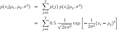
where j indexes the two normal distributions (µ1 and µ2 are their means and σ 2 is their common variance).
Hint: Just like in Part (b), you’ll need two subchains, one for the mean of the first distri-bution, and the other for the mean of the second distribution. And, again just like in Part (b), the two subchains are linked. For instance, when you evaluate a proposed sample for the first mean, you’ll need to calculate the likelihood based on this proposed sample. To do so, you’ll need a value for the second mean. For this, you should use the most recent sample value from the subchain for the second mean. This illustrates that the subchain for the first mean is linked to the subchain for the second mean. In an analogous way, the subchain for the second mean is linked to the subchain for the first mean.
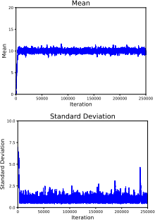
Figure 3: Results of running the Metropolis-Hastings (MH) algorithm to estimate both the mean and the standard deviation of a normal distribution from a dataset of 10 values sampled from that distribution (see Question 3, Part B).
2025-04-17