MAT3007 · Homework 11
Hello, dear friend, you can consult us at any time if you have any questions, add WeChat: daixieit
![]() MAT3007 · Homework 11
MAT3007 · Homework 11
Instructions:
• Homework problems must be carefully and clearly answered to receive full credit. Complete sentences that establish a clear logical progression are highly recommended.
• You must submit your assignment in Blackboard. Please upload a zip file including your answer and code. The file name should be in the format last name-first name-hw11.
• The homework must be written in English.
• Late submission will not be graded.
• Each student must not copy homework solutions from another student or from any other source.
Problem 1 Gradient Descent Method(30pts).
Implement the gradient descent method in MATLAB to solve the optimization problem:

The following input parameters should be considered:
• x0 = (0, 0)⊤ – the initial point.
• tol = 10 −5 – the tolerance parameter. The method should stop whenever the current iterate xk satisfies the criterion ∥∇f (xk )∥ ≤ tol.
• σ, γ = ![]() – parameters for backtracking and the Armijo condition.
– parameters for backtracking and the Armijo condition.
Implement different methods using the given parameter.
a) Implement the gradient descent method using constant stepsize. Choose α1 = 1 and α2 = 0.1, report the number of iterations, the final objective function value, and the point to which the methods converged.
b) Implement the gradient descent method using exact line search method, report the number of iterations, the final objective function value, and the point to which the methods converged.
Hint: You can use golden section in exact line search.
c) Implement the gradient descent method using backtracking (Armijo) line search method, report the number of iterations, the final objective function value, and the point to which the methods converged.
d) Plot figures of the solution path for each of the different step size strategies (similar to the one in the lecture slides).
Please include (1) essential parts of code (2) output results and figures in your answer.
Problem 2 Newton’s Method(20pts).
Implement the Newton’s method in MATLAB to solve the same problem in Problem 1.
Use only Armijo backtracking line search. Report the number of iterations, the final objective function value, the point to which the methods converged. Plot figures of the solution path.
Hint: Matlab has functions for matrix inversion
Problem 3 Projection Theorem (30pts)
Consider the projection problem
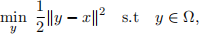
where Ω is nonempty, closed, and convex. Let y∗ be the unique minimizer and we define the projection operator y∗ = PΩ(x). In this exercise, we would like to derive some nice properties of the projection operator PΩ(·).
(a) Show that y∗ = PΩ(x), if and only if

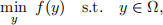
Hint: This result is the so-called projection theorem. It characterizes fully projection geometry. To prove this projection theorem, you can use the following FONC for convex constrained optimization problem (you can use it without proving it. Indeed, if you are interested, you can try to prove it using the theorem on page 14 of slides 15): consider miny f (y) s.t. y ∈ Ω, where Ω ⊂ Rn is a convex and closed set and f is cont. diff. on an open set containing Ω, the FONC of this problem is given by ∇f (y∗)⊤(y − y∗) ≥ 0, ∀ y ∈ Ω with y∗ being a local minimizer.
(b) In our development of the projected gradient method, the theorem on page 25 of slides 23 said that the generalized gradient d := PΩ(x − λ∇f (x)) − x is a descent direction. In its proof, the first inequality on page 26 of slides 23 is not one step justification. In order to justify this step, let us use part (a) to show

In addition, show that the projection operator PΩ(·) is 1-Lipschitz continuous.
(c) The stopping criterion in the projected gradient method is ∥d∥ ≤ ϵ for some small enough ϵ . To justify this criterion, using the result and the hint in part (a) to show that x∗ is a stationary point of
if and only if

Problem 4 Branch-and-Bound Method (20pts)
Use the branch-and-bound method to solve the following integer program.
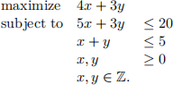
You are allowed to solve each of the relaxed linear program by MATLAB. Please specify the branch- and-bound tree and what you did at each node.
2021-12-23