Exam. Survival analysis 2024-2025
Hello, dear friend, you can consult us at any time if you have any questions, add WeChat: daixieit
Exam. Survival analysis 2024-2025
Question 1
Assume that the hazard of the event time T* is related to the bounded continuous scalar covariate x by
α(t|x = ∞) = α0 (t) + θ∞
where α0 (⋅) is a continuous baseline hazard function and the covariate effect θ ∈ Θ, where Θ is a bounded interval, does not depend on time.
In (a)−(d), consider T* observed subject to independent and non-informative right- censoring by c, following a distribution with continuous hazard αc, in the bounded interval [0, T]. We observe (Ti = Ti* ∧ ci , Δi = I{Ti* ≤ ci}, xi) for i = 1, … , n, independent subjects and Ti* ⫫ ci |xi . Let yi (t) = I{Ti ≥ t}. Under these conditions, for k a non-negative finite integer, 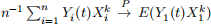 uniformly in t ∈ [0, T] and E(y1 (t)) is bounded away from zero for any t ∈ [0, T].
(a) Let Ni (t) = I{Ti ≤ t, Δi = 1} and Mi (t) = Ni (t)− yi (s)α(s|xi)ds. Argue
that
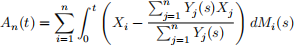
is a mean zero martingale (specify what filtration you are considering). Show that n—1/2An (t) converges weakly to a Gaussian martingale.
(b) Use the martingale property from (a) to argue that
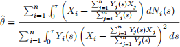
is a reasonable estimator of θ .
(c) Show that n1/2 (θ − θ) is asymptotically normally distributed and suggest an
estimator of the standard error of θ .
(d) Suggest an estimator of the cumulative baseline hazard α0 (s)ds. You don’t
have to derive the distribution of the estimator.
In (e)−(f), consider the same hazard of T∗ as above, but a very different observation scheme, that will require another estimation strategy. Let ui be an inspection time following a distribution with hazard αu(t) and be independent of Ti∗ and xi . At time ui it is investigated whether the event of interest has happened to individual i or not. The observed data is (I{Ti∗ ≥ ui}, ui , xi) for i = 1, … , n independent individuals. Note that the exact event times Ti∗ are never observed.
(e) Consider a realized inspection time ui = u for an individual with covariate xi = ∞ . What is the probability that the individual has not experienced the event yet at time u?
(f) Let Ni (t) = I{ui ≤ t,Ti∗ ≥ ui}, indicate that subject i was investigated before or at time t, and that it was found that they had not yet experi- enced the event at the inspection time. Let yi (t) = I{ui ≥ t}. What is the intensity of the counting process Ni with respect to the filtration ℱt = σ(Ni (s), yi (s), xi ; i = 1, … , n, s ≤ t)?
(g) Suggest an estimating equation for estimating θ . It is enough to specify and motivate the equation, you do not need to show any properties or consider how to solve it.
Question 2
Consider a competing risk setting with two competing causes of death. Let T∗ denote the time to death and ε the cause of death. We are interested in the cause 1-specific hazard ratio for a scalar bounded covariate x. However, for some individuals the time to death is observed, but not the cause of death, for others both the time and cause is observed. Let R = 1 denote that the cause of death was observed and R = 0 that it was missing. The events are observed in the time-window [0, T], T < ∞, subject to independent and non-informative right-censoring (conditioning on x) at time c (following a distribution with continuous hazard). We observe the data
(Ti = Ti∗ ∧ ci , Δi = I{Ti∗ ≤ ci}, Ri , xi , Ri Δi εi)
for i = 1, … , n independent individuals.
Let αk , k = 1, 2, denote the cause k-specific hazard, and let α• = α 1 + α2 denote the all cause hazard. We assume that they are continuous and that they have the form
α 1 (t|x = ∞) = α0 (t) exp(β∞)
α2 (t|x = ∞) = α0 (t)q2 (t, ∞),
where q2 (t, ∞) is a known function that doesn’t involve unknown parameters. To ease notation, let
q• (t|x = ∞; β) = exp(β∞) + q2 (t, ∞)
such that
α• (t|x = ∞) = α0 (t)q• (t|x = ∞; β).
Let π denote the probability that the cause of death is observed. Conditionally on that the individual was observed to die, the covariate and the time of death, we assume that the missingness probability does not depend on the cause of death itself,
pr(R = 1|Δ = 1,T, X, ε) = pr(R = 1|Δ = 1,T, X) = π(T, X).
(a) Consider the counting processes
N1i (t) = I{Ti ≤ t, Ri Δi εi = 1}
N2i (t) = I{Ti ≤ t, Ri Δi εi = 2}
NMi (t) = I{Ti ≤ t, (1 − Ri)Δi = 1}
indicating that a death from cause 1, 2 or an unknown cause has been observed by time t. Define the filtration
ℱt = σ(N1i (s), N2i (s), NMi (s), yi (s+), Xi , i = 1, … , n, s ≤ t)
where yi (t) = I{Ti ≥ t}. Argue why the intensity of Nki (t) with respect to ℱt is yi (t)π(t, Xi)αk (t), for k = 1, 2 and that the intensity of NMi (t) with respect to ℱt is yi (t)(1 − π(t, Xi))α• (t). Find also the intensity of the all cause-counting process N•i (t) = I{Ti ≤ t, Δi = 1}.
(b) Write up the likelihood of (α0 (⋅), π(⋅, ⋅), β) based on the observed data in [0, T] from the n individuals.
(c) For fixed β, the cumulative baseline hazard Α0 (t) = α0 (s)ds can be estimated
by the Breslow estimator
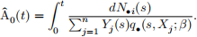
Write up the profiled likelihood obtained by replacing α0 (t) in the likelihood from
(b) by ΔΑ(t), the jump of the Breslow estimator at time t. Note that the Breslow estimator is a step function with jumps only at the uncensored death times.
(d) The (profiled likelihood) score for β using information up to time t ≤ T is
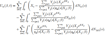
Show that un (β,t) is a martingale with respect to ℱt .
By Rebolledo’s central limit theorem, n−1/2un (β,t) evaluated at the true value of β , converges to a Gaussian martingale with variance σ 2 (t) as n → ∞ (you don’t have to show this).
(e) Show that the expectation of the observed information
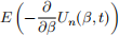
equals the expectation of the predictable variation of the score
E (⟨un (β, ⋅)⟩(t))
when evaluated at the true value of β .
It is further possible to show that −n−1 un (β,t) and ⟨n−1/2un (β, ⋅)⟩(t) converges to the same limit in probability, and that for ![]() = β +OP(1), it holds that n−1 un (β, T)∣β=
= β +OP(1), it holds that n−1 un (β, T)∣β=![]() = n−1
= n−1 ![]() un (β, T) + OP(1). You don’t have to verify this.̂
un (β, T) + OP(1). You don’t have to verify this.̂
(f) The solution β to un (β, T) = 0 is a consistent estimator of β (you don’t have to show
![]() this). Show that n1/2 (β − β) is asymptotically normally distributed and suggest
this). Show that n1/2 (β − β) is asymptotically normally distributed and suggest
an estimator of the variance of β that doesn’t require estimating the missingness probability π .
Question 3
In this question you will implement the estimator from Question 2. The R code below will simulate n = 400 competing risk observations on [0, T], T = 1, from the cause specific hazards
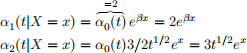
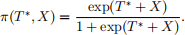
where β = 0.5 and X is uniformly distributed on [0, 1], subject to censoring with hazard αc = 1. For an uncensored death time T∗ from an individual with covariate X, the cause of death (1 or 2) is missing with probability
n <- 400
beta0 <- .5
x <- runif(n)
T1 <- -log(runif(n))/(2*exp(beta0*x))
T2 <- (-log(runif(n))/(2*exp(x)))^(2/3) C <- rexp(n,1)
tau <- 1
obstime <- pmin(T1,T2,C,tau)
status <- 1*(obstime==T1) + 2*(obstime==T2)
status[(runif(n)
The information that you will use is
• obstime : the time to censoring or death, whichever came first
• status : 0; censoring, 1; dead cause 1, 2; dead cause 2, 3; dead unknown cause
• x : the covariate X
Note that we assume that
is fully known and given to us. However, β , α0 (t) and π(t, ∞) are not known.
In (a) − (c) you will use a single data set of size n = 400 generated with the code above, using the seed 9525, i.e. set the seed with set.seed(9525) before simulating the data. In (e) you will generate 1000 different data sets. In each step, describe what you are doing and why. Only R code is not enough.
(a) Implement the score of β from Question 2(d). Simulate one data set with the seed specified above. Evaluated at β = 0.5 the score should be −2.214685 for this seed.
(b) Estimate β by solving the score from (a) for 0, i.e., implement the estimator from Question 2(f). Also estimate the standard error of the estimator and calculate the 95% confidence interval. Report the result. You may use any numerical solver and make use of numerical derivatives. You may for example use the solver nleqslv that finds the root of a function and returns the derivative of the function evaluated at the solution (if you set the option jacobian=TRUE).
(c) Implement the estimator of the cumulative baseline hazard from Question 2(c). Apply the estimator to the simulated data set and present it in a plot. Compare it to the data generating ds = 2t.
(d) Use your estimators from (b) and (c) to estimate the absolute risk (cumulative incidence) for a type 1 event for an individual with covariate X = 0.8, i.e., F1 (t|X = 0.8) = pr(T∗ ≤ t, ε = 1|X = 0.8). Also plot the true (data generating) absolute risk function. Making use of numerical integration is allowed.
(e) Perform a simulation study where you simulate 1000 data sets each of size n = 400 and apply your estimator from (b) to each of these data sets to estimate β, its standard error and a 95% confidence interval for it. Also use a standard Cox model to estimate β treating only the observed cause 1 deaths, i.e., status=1, as events, while deaths from an unknown cause status=3 are treated as censorings.
Report the average of the estimated βs, the standard deviation of the estimated βs, the average of the estimated standard errors and the percentage of times the true value β = 0.5 is contained in the estimated confidence intervals. Conclude.
2025-01-17