Hello, dear friend, you can consult us at any time if you have any questions, add WeChat: daixieit

7SSG5110 Methods in Environmental Research

Practical 9: Sampling Statistics

Introduction

In this practical we will use Excel and R to explore some of the concepts regarding statistics for sampling discussed in the lecture. Before you start the activities below, create a working directory for this practical (e.g. N:/My Documents/Practical). Files we will use in this practical are available in the KEATS space.

Part 1: Sample size and confidence intervals (Excel)

Joe, Ahmed, Kim, Sally and Miguel want to estimate the species richness of birds in a forest. They used fixed-radius point counts at random locations in the forest, counting the number of species they saw or heard in a 5-minute period within 20m of where they were stood. The number of times they did their 5-minute counts (i.e. their sample size) varied. The data collected by these students can be found in BirdSampling.xlsx.

To understand the uncertainty in these data, we will use Excel to calculate and plot mean and 95% confidence intervals (CI) for their estimates of forest bird species richness. A sheet named ‘Working’ has been provided for you in which you can calculate values (this sheet has a structure which will make it easy to later plot your calculations).

Your first calculation is the Standard Error (SE) for the students’ sample data:

 Eq. 1

where s is the sample standard deviation and n is the sample size. Once you have calculated the SE you can use Eq. 2 to calculate a confidence interval (CI):

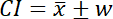 Eq. 2

where:

 Eq. 3

and where w is the Margin of Error and z is the z-score for the level of confidence you want to use (e.g. see Cumming and Finch 2005). For example, z for 95% confidence is 1.96 and z for 99% is 2.58. In conjunction with the sample mean (), we can define the upper and lower confidence limits:

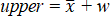  Eq. 4a

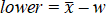 Eq. 4b

Row titles have been suggested below the students’ data in the Excel spreadsheet provided. To make the necessary calculations in Excel you will need to use combinations of the following functions: average(), count(), stdev() and sqrt().

Once you have calculated your values use them to complete Table 1 (copy the values in this Word document) as a summary of the students’ surveys.

Q1. Using your completed Table 1, answer the following questions (type your answers):

a) Which student has the least certain species richness estimate?

b) Which student do you think has the best estimate of species richness?  

c) How do the 95% CI values vary by student? What is this related to?

Table 1. Results from student bird survey

Next, create a scatter plot in Excel with Sample Size on the x-axis and Species Richness estimate on the y-axis. Format your plot appropriately with axis labels, etc. To visualise the uncertainty in the students’ estimates of species richness we will add ‘error bars’ (also known as ‘whiskers’) to the plot. Use the following steps to do this in Excel:

1. Select the chart you have created, then click the ‘Design’ tab that will appear in the menu

2. Click ‘Add Chart Element’ button on far left of the ribbon and select Error Bars -> More Error Bar Options… [You will see several pre-configured options (e.g. Standard Error) but we will use the confidence intervals we have calculated ourselves.]

3. A ‘Format Error Bars’ pane will appear on the right of the screen. Initially Excel adds error bars in both vertical and horizontal directions. We will delete the horizontal bars later as we only want vertical here (Think why this is?)

4. We will add bars in both positive and negative directions using a custom value (our 95% confidence intervals); select the ‘Custom’ radio button at the bottom of the ‘Format Errors Pane’ and click ‘Specify Value’

5. Select the 95% CI values for each student for both positive and negative error values (click the red arrow then click and drag, click the red arrow again, then click done). Click Close on the Format Error Bars dialogue box.

6. We have now added vertical error bars indicating the 95% confidence interval for each student’s estimate of Species Richness. To remove the horizontal bars, click on one of the horizontal error bars in the chart and press ‘delete’ on the keyboard.

You can add ‘error bars’ (indicating uncertainty) like this to other charts in Excel (e.g., bar charts).

Now, let’s assume that Joe is unhappy with his estimate of species richness. He wants to know how many samples he should take to get an estimate of species richness ± 1 species (at the 95% level of confidence). This can be calculated using Eq. 4:

 Eq. 4

where z is the z-score for the corresponding level of confidence, σ is the sample standard deviation and w is the acceptable margin of error.

Q2. Using Eq. 4 in Excel and the values you have entered in Table 1, answer the following questions:

a) What is z for the 95% confidence interval?

b) What are you going to use as your estimate of σ (assume Joe has seen your completed Table 1)?

c) What is Joe’s acceptable margin of error, w (this was specified in the text above)?

d) Consequently, for the values for z, σ and w you have decided to use, what is the minimum number of species counts should Joe make?

Part 2: Sample size and testing for differences.

In this part we will us R to explore the effects of sample size on the confidence interval and on detecting differences. Some of the code in this practical will be familiar, other code shows you some more examples of manipulating data in R.

We will use the packages tidyr and ggplot2. So the first step is to clean the workspace and load the required packages (note that you will have to install the packages first if they are not installed already).

rm(list=ls())

library(tidyr)

library(ggplot2)

We start by generating some data for two imaginary locations loc1 and loc2. We generate "observations" from a normal distribution. We specify the mean and standard deviation of the distribution that we want to sample from. We use the same standard deviation for our two locations, but we use different means. Thus, we know, that in our generated reality, loc1 and loc2 have different means.

We use set.seed() to set the seed for our random number generator. By setting the seed, we ensure that each time we generate random observations with rnorm(), they are the same values. You can read more by typing ?set.seed in the console. This is useful if you want to generate random numbers, but you want to be able to replicate those exact same random numbers in the future.

set.seed(3)

loc1 <- rnorm(1000, mean=20, sd=5)

loc2 <- rnorm(1000, mean=22, sd=5)

 

We then create a data frame that includes the data for the two locations and transform it to the long format, so we can use ggplot for plotting.

dat <- data.frame(loc1=loc1, loc2=loc2)

location.data <- gather(data = dat, key = Location, value = Observation)

Let’s have a look at the data, plot the data for the two locations and compare the distributions.

Q3. Comparing the data for the two locations, what do you notice?

#We can do this using a boxplot

plot1 <- ggplot(location.data, aes(x=Location, y=Observation))

plot1 + geom_boxplot() + ylab("Observation")

#Or a histogram

plot2 <- ggplot(location.data, aes(Observation))

plot2 + geom_histogram(binwidth = 5) + facet_grid(Location ~ .)

Now we are going to investigate the influence of sample size on the ability to detect differences. We divide the data into different samples for the two locations. We do this for a sample size of 10 and 100.

To divide the data into different sample groups, we first have to create a vector that for each entry in the data frame gives the group that entry will belong to. Have a look at the output of the following code (i.e. print sample.groups.10) and also have a look at the output of rep(1:100,each=10). Do you understand what is happening?

sample.groups.10 <- rep(rep(1:100,each=10),times=2)

sample.groups.100 <- rep(rep(1:10,each=100),times=2)

Now we can use the vectors with groups to divide our location.data into different samples. To understand how this works, you can have a look at what the data frame location.data looks like, what sample.groups.10 looks like and you can read the help by typing ?split in the console.

samples.size10 <- split(location.data, f = sample.groups.10)

samples.size100 <- split(location.data, f = sample.groups.100)

As you can see samples.size10 and samples.size100 are lists that contain several data frames. You can access something in a list by using double square brackets, like this: samples.size10[[1]]. This will give you the first entry of the list. In this case the first sample with ten observations for loc1 and ten observations for loc2. (Print the data frame and some of the entries to make sure you understand.) Lists are objects in R, that can contain other objects, such as data frames, vectors, matrices and also other lists. Each entry in a list can be different, for example, the first entry can hold a vector, while the second entry holds a data frame.

We now want to calculate some statistics for each of our samples (i.e. for each of the data frames in our list).

We can apply the same function to every entry in a list efficiently, by using lapply or sapply. We are going to do this now to calculate some statistics for each of our samples. First, we are defining the function that we want to apply.

sample.stats <- function(x){   

  x1 <- x$Observation[which(x$Location=="loc1")]

  x2 <- x$Observation[which(x$Location=="loc2")]

  mean1 <- mean(x1)

  mean2 <- mean(x2)

  sd1 <- sd(x1)

  sd2 <- sd(x2)

  se1 <- sd1/sqrt(length(x1))

  se2 <- sd2/sqrt(length(x2))

  CImin1 <- mean1-se1*1.96

  CImin2 <- mean2-se2*1.96

  CImax1 <- mean1 + se1*1.96

  CImax2 <- mean2 + se2*1.96

  return(c("mean1" = mean1, "sd1" = sd1, "se1" = se1,

           "CImin1" = CImin1, "CImax1" = CImax1,

           "mean2" = mean2, "sd2" = sd2, "se2" = se2,

           "CImin2" = CImin2, "CImax2" = CImax2))

}

Now we can use sapply to calculate the summary statistics for each data frame in our list.

We provide the list (sample.size10) and we specify the function that we want to apply (sample.stats).

sum.stats <- sapply(samples.size10, FUN=sample.stats)

Print sum.stats and have a look at the output. Do you understand what sapply did?

For plotting in ggplot we transpose the matrix and transform it into a data frame. We also add some labels to use for plotting. paste() will paste together several lines of characters and numbers, you can read the help page (write ?paste in the console) for more info.

sample.stats.size10 <- as.data.frame(t(sum.stats))

sample.stats.size10$Sample <- seq(1,100) #we add a sample number

sample.stats.size10$lab <- paste("Sample ",seq(1,100))

We repeat the same thing for the samples of size 100.

sample.stats.size100 <- as.data.frame(t(sapply(samples.size100, sample.stats)))

sample.stats.size100$Sample <- seq(1,10)

sample.stats.size100$lab <- paste("Sample ",seq(1,10))

Now we also want to know what the effect of the sample size is on being able to tell the difference between the samples for location 1 and location 2. In other words, we want to know the effect on the performance of a t-test. To do that we define a function that applies the t.test function but only returns the p.value.

list.t.test <-function(x) {

  return(t.test(Observation ~ Location, data=x, var.equal = TRUE)$p.value)

}

In the same way that we calculated the summary statistics for our different samples, we apply the list.t.test function to each data frame in our list. We do this for both the samples of size 10 and of size 100. And we then add these values to the data frames with sample statistics.

tt.ss10 <- sapply(samples.size10, list.t.test)

tt.ss100 <- sapply(samples.size100, list.t.test)

sample.stats.size10$tt <- tt.ss10

sample.stats.size100$tt <- tt.ss100

Now let's have a look at our results. The following code creates a graph that shows the mean and 95% confidence intervals for each set of samples. We also plot the p-values of the t-test performed for each sample pair. Plot3 is for the samples of size 10 and plot 4 for the samples of size 100.

The code below provides a lot of examples of how to tweak your plot in ggplot. We use geom_pointrange() which allows us to plot points for the mean, with lines indicating the confidence interval. The r file that contains the entire code of this practical part 2 provides some annotations that may help you understand what each part of the code does.

plot3 <- ggplot(data=sample.stats.size10[1:10,], aes(x=1, y=mean1, ymin=CImin1, ymax=CImax1))

plot3 + geom_pointrange() +

  coord_flip(xlim=c(0,1.5), ylim=c(15,30), clip="off") +  

  labs(x = NULL, y="Mean (95% CI)") +

  geom_pointrange(aes(x=0.5, y=mean2, ymin=CImin2, ymax=CImax2, color = "darkred")) +

  facet_grid(Sample ~ .,switch="y",

             labeller = labeller(Sample = sample.stats.size10$lab)) +

  theme(axis.text.y=element_blank(),axis.ticks.y=element_blank(),

        axis.title.y=element_blank(),axis.line=element_line("black"),

        panel.background=element_blank(),

        panel.border=element_rect(color="grey", fill="NA",linewidth=0.1),

        panel.grid.major.x=element_line("grey"),

        panel.grid.minor.x=element_line("grey"),

        panel.grid.major.y=element_blank(),panel.grid.minor.y=element_blank(),

        plot.background=element_blank(),

        strip.background = element_rect(color="black",fill="white"),

        strip.text.y.left = element_text(angle = 0), legend.position="NA",

        plot.margin = unit(c(3.5,5.5,1,1),"lines")) +

  geom_text(aes(x = 1, y = 33, label = round(tt[1:10],3)+

  geom_text(aes(x = 2.5, y = c(14), label=c("Sample", rep("",9))))+

  geom_text(aes(x = 2.5, y = c(23),

                label=c("Mean of samples at loc 1 (black) and 2 (red) (n=10)", rep("",9                ))))+

  geom_text(aes(x = 2.5, y = c(32.5), label=c("p-value of t-test", rep("",9))))

plot4 <- ggplot(data=sample.stats.size100[1:10,], aes(x=1, y=mean1, ymin=CImin1, ymax=CImax1))

plot4 + geom_pointrange() +

  coord_flip(xlim=c(0,1.5), ylim=c(15,30), clip="off") +  

  labs(x = NULL, y="Mean (95% CI)") +

  geom_pointrange(aes(x=0.5, y=mean2, ymin=CImin2, ymax=CImax2, color = "darkred")) +

  facet_grid(Sample ~ .,switch="y",

             labeller = labeller(Sample = sample.stats.size10$lab))+

  theme(axis.text.y=element_blank(),axis.ticks.y=element_blank(),

        axis.title.y=element_blank(),axis.line=element_line("black"),

        panel.background=element_blank(),

        panel.border=element_rect(color="grey", fill="NA",linewidth=0.1),

        panel.grid.major.x=element_line("grey"),

        panel.grid.minor.x=element_line("grey"),

        panel.grid.major.y=element_blank(),panel.grid.minor.y=element_blank(),

        plot.background=element_blank(),

        strip.background = element_rect(color="black",fill="white"),

        strip.text.y.left = element_text(angle = 0), legend.position="NA",

        plot.margin = unit(c(3.5,5.5,1,1),"lines")) +

  geom_text(aes(x = 1, y = 33, label = round(tt[1:10],3))) +

  geom_text(aes(x = 2.5, y = c(14), label=c("Sample", rep("",9)))) +

  geom_text(aes(x = 2.5, y = c(23),

                label=c("Mean of samples at loc 1 (black) and 2 (red) (n=100)",

                rep("",9))))+

  geom_text(aes(x = 2.5, y = c(32.5), label=c("p-value of t-test", rep("",9))))

Q4. Have a look at the plots that you have just created and compare plot 3 and plot 4. What differences do you notice when looking at the confidence intervals? What differences do you notice when looking at the p-values? How are the two related?

Now that you have the code in R, you can explore how these effects change for smaller or larger differences in the mean or for smaller or larger standard deviations (i.e. vary the means and standard deviation of the datasets that you generated at the start of part 2).

Part 3: Optional: sample size and sample timing

Part 3 of this practical explores the effect on the analysis of sample size and sample timing, see the R code provided in the SamplingInR_Tiree.r R script available on KEATS. This R script shows how data can be sampled from a climate data set (TireeClimate.csv also on KEATS). These data are for Tiree, an island off the west coast of Scotland, and are from MetOffice (2013) and should be downloaded from KEATS to your hard drive for use in R. Details of how the R script works are not provided here, and you should review the code and the comments that accompany it to identify and understand what the code in the script does and how it works (examining and playing with other people’s code, in conjunction with help functions and the internet, is one of the best ways to learn R). Remember you can review how to use scripts in R in the Overview of R document on KEATS.

References Cited

Cumming, G. and Finch, S. (2005). Inference by Eye: Confidence Intervals and How to Read Pictures of Data. American Psychologist 60(2), 170

MetOffice (2013) Historic Station Data [Online] Available from: http://www.metoffice.gov.uk/public/weather/climate-historic/ [Accessed 15^th October 2016]