Hello, dear friend, you can consult us at any time if you have any questions, add WeChat: daixieit

CHE421

Coursework Assessment 2

Exercise

Use of AI in Problem Solving: Students are required encouraged to use AI tools as part of their problem-solving process for this assessment.

These Projects are worth 75 marks only. There are an additional 25 marks available for the evaluation of your use of AI in answering these exercises.

In doing so, you should:

(a)  Clearly explain why any corrections or adjustments were necessary, referencing the relevant principles covered in lectures.

(b)  Provide  evidence  of  their  own  reasoning  and  understanding,  showing  how  they applied course content to improve or verify AI's suggestions.

(c)  Thoughtfully balance the AI’s utility with their own critical analysis.

For each of Project 1 and Project 2, submit a transcript of your interaction with AI for each question (e.g., cut and paste into a word document called “AI interactions.docx”) together with a critical evaluation of your interaction with AI addressing the three points above. [25 marks]

Project 1

Mapping the potential energy surface for the co-linear reactive collision of a fluorine atom with a hydrogen molecule:

F(g) + H2(g) - HF(g) + H(g)

Potential energy surfaces may be used to map chemical reactions. In this project you will map potential energy surfaces for the following reaction:

F(g) + H2(g) - HF(g) + H(g)

The reaction proceeds via an [F-H-H]* activated complex, and then one of the hydrogen atoms departs leaving an HF molecule behind. Assume that the reaction occurs co-linearly. That is, the F atom approaches the H2 molecule along the C。 axis of the molecule.

The potential energy surface for reaction (1) may be represented by a 3-D plot with the H-H separation on the x-axis, the H-F separation on the y-axis, and the electronic energy (in electron volts) on the z-axis.

(a) Generate this potential energy surface calculated at CCSD level using an appropriate for the problem and present a 3-D graph of the potential energy surface for this reaction in your answer (make it big – full A4 page).

Separately submit all input files used, and output files you generated ‘zipped’ into a single file called “1A.zip”.

Hint: You are likely to encounter problems with bond lengths being too short and too long for Gaussian to deal with. You will need to ‘experiment’ with your input file to find appropriate minimum and maximum values. However, each scan should not take more than 10 minutes even with the biggest possible basis set for the problem).

You will also need to choose a step size that will give an informative graph of the PES. The finer the step size, the more informative the graph. But the number of data points scales with the square of the number points alone each axis (e.g., rough grid (10x10 points) gives 100 points to be extracted from the output file and entered into Excel. 50x50 grid give 2500. There is enough time given to this exercise to do this manually. However, you may find AI helpful in generating a method (e.g., via a script) to automatically extract the data in a fraction of a second and automatically generate a comma separate variable (CSV) file that maybe opened in Excel to then generate the 3D PES plot. A 10,000-point 100 x 100 plot is not unreasonable if AI, or other expertise, is used.

Project: 2

Molecular Simulations of Water

Overview:

In this project we will perform a simulation of 300 water molecules. After that, you will write a small tool that calculates the radial distribution function using python. For that you will make use of the trajectory file you obtained using the MD simulation.

Perform water simulation

Download the corresponding file from Learning Mall. The archive folder contains three files. The first file called *water_lammps.inp* defines the conditions of our simulation, which contains the parameters for non-bond, bond and angle potentials. The water model is often referred to as the SPC/E (extended simple point charge) flexible water model. The second file *SPCE_water.data* contains the mass, charge and position of all atoms. It also tells the code how the atoms are connected by bonds and angles. Copy both files to your working directory and start the simulation, with a command similar to the one written below.

lmp_serial -in water_lammps.inp

The simulation should finish within ~30 minutes if run on 1 core, as described here. After that, open the dump file *water.dump*. It contains 201 frames that were taken every 500 timesteps. A small header section reads the timestep, number of atoms and the simulation cell size for each frame in Angstrom.  If the simulation takes  longer (or you can  not successfully run the simulation) you can still start programming in the analysis script. The third file *example.lammpstrj* gives you an impression on the format that is used to write the trajectory.

Questions:

(a)  Write down the force-field functional form of the bond interaction used to model the water system [2 marks]

(b)  Perform the lammps simulation of water with provided input files and obtain the output files including file *water.dump* with require information and file *oxygen.rdf*. [3 marks]

Watch the progression of your trajectory

Type ```vmd``` in the terminal. This opens up 2 windows. We will still use the terminal to load our initial configuration and bond connectivity. In the terminal type (remember your directory paths!)

topo readlammpsdata SPCE_water.data

Now that we have the initial configuration and the bond connectivity, it is time to load our trajectory and see how our simulation visually looks and progressed like.

In the window of VMD, click on **File** and then **New Molecule**.... In Load files for: select *SPCE_water.data* (select the previously loaded initial configuration in the drop down menu), click on **Browse**... (select *water.dump*) and select **Determine file type**: as LAMMPS Trajectory in the drop-down menu. Then click on Load. Once loaded you can use the ”VMD main” main window to control and see how your simulation has progressed. You can explore options like selecting certain atoms/molecules and colouring them differently or using different representations like beads, lines, ribbons etc. found in **Graphics and Representations**...

Questions:

(a)  Open VMD and load the data file correctly, make a snapshot that includes all windows associated with VMD software:

(i)   VMD main,

(ii)  Molecule File Browser,

(iii) VMD Display,

(iv) Graphical Representations [6 marks]

(b)  Render the water beads with CPK representation. [2 marks]

(c) Load file *water.dump* for water [water.dump/example.dump], make a snapshot that  includes all windows required in previous question. [2 marks]

Radial distribution function (rdf)

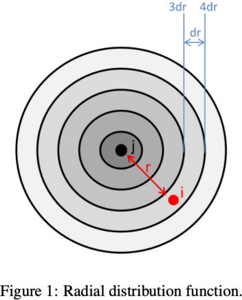
The rdf is the normalized number density of particles i with distance to another particle j. This means that one has to count how many particles i are inside a radial shell of a predefined slab size with a thickness dr around a particle j with a distance of r. Division of this number by the volume element of this shell gives you the number density. At the end you must normalize this density by the bulk density to get the normalized radial distribution function. Figure 1 illustrates the situation. Use the trajectory file from the water simulation to calculate the rdf for all pairs of oxygen-oxygen.

For this, write a program, based on the code prepared: *rdf_basic.py*, that reads the positions of all oxygen atoms and save them in an array. Then for each frame, loop over all oxygen j and measure the distance to all other oxygen atoms i. You will need three loops for that. Once you have the distance, you must determine the slab where atom i is located.  Remember  that  the   coordinates   in  your  trajectory  file   are  unfolded  box coordinates.  However,  for the  radial  distributions function you  need  to  calculate the distance according to the closest image convention. As a consequence two atoms cannot be further away than half of the box length. Save your result in a histogram that counts the number of atoms found in each shell and print out the average at the end. Later you can refine the code and divide by the shell volume and the bulk density.

Hint: you can always compare your resulting rdf to *oxygen.rdf* which will be created by LAMMPS when you finished your simulation.

Question:

(a)  Describe the basic procedure of the rdf algorithm before you start writing the program itself. [5 marks]

Hint: To dramatically speed up your pbc treatment look into numpy’s ”where” method (np.where). And remember that arrays can be accessed with a list of indices.

(b)  Write down the mathematical equation for calculating the radial distribution function. [5 marks]

(c)  Supply your source code for calculations of the radial distribution function of

oxygen-oxygen, with your calculated RDF plotted together with LAMMPS output. [5 marks]