EMAT20920: Numerical Methods in MATLAB
Hello, dear friend, you can consult us at any time if you have any questions, add WeChat: daixieit
Department of Engineering Mathematics
EMAT20920: Numerical Methods in MATLAB
COURSEWORK ASSESSMENT
Question 1: Root-finding
(a) Find all the solutions of the following equations in the given intervals, accurate to 14 significant
figures, using built-in Matlab commands. In all cases, you should give sufficient evidence for your answers, and state:
• the number of solutions in the interval,
• the values of the solutions,
• the Matlab command(s) used to find them.
(i) tan3(x) + π = cot(x), for −2π ⩽ x ⩽ 2π ,
(x − 2)2 p|x + 3| = e −x4/9, for −2π ⩽ x ⩽ 2π ,
(iii) Z0m x2 e −x/2 dx = 8, for 0 ⩽ m < ∞,
(6 marks)
(b) Consider a root-finding method that finds solutions of f(x) = 0, for a function f : R 7→ R, by
successively refining a bracketing interval as follows:
• Suppose that [a,b] is a bracketing interval.
• Compute m and n, two candidate endpoints for a new bracketing interval1, as follows:
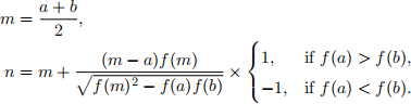
• If f(m) and f(n) are of opposite sign then use n and m as the endpoints of the new bracketing interval.
• Else, use
◦ a and n, if f(a) and f(n) are of opposite sign,
◦ n and b, if f(b) and f(n) are of opposite sign
as the endpoints of the new bracketing interval.
(i) Write a Matlab function that uses the algorithm above to find a root x⋆ of a given function f , to a desired tolerance ϵ, given an initial bracketing interval [a,b]. Together with your function, you should describe any tests you have used to ensure that it works correctly.
(6 marks)
(ii) Use your function to find the order of the root finding method — giving appropriate evidence — when used to find roots of the function f(x) = e −x −x in the interval x = [0, 2], correct to 14 d.p.
(3 marks)
(iii) Describe the strengths and weaknesses of the method, in comparison to the bisection and
Newton-Raphson methods.
(1 mark)
(c) For what values of k will the fixed-point iteration
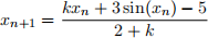
converge?
(4 marks)
![]()
Question 2: Numerical integration and differentiation
(a) Write a Matlab function that uses Simpson’s rule to find the value of the function F given by
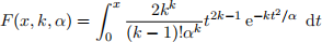
correct to 8 decimal places, given values x > 0, α > 0, and k ∈ Z with k > 0. Use your code to plot a single graph of F(x,k,α) as a function of x, for values k = 1, 2, 3 and α = 1, 2, 3.
(6 marks)
(b) The expression
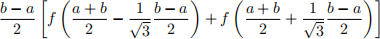
can be used to approximate the integral R![]() f(x) dx.
f(x) dx.
Write a MATLAB function that calculates a numerical approximation to an integral R![]() f(x) dx
f(x) dx
using a composite version of equation (1) with N panels; i.e., where the interval [α,β] is divided into N equal-width intervals of width h = (β − α)/N, on each of which we use equation (1).
Use your function to find
(i) The number of panels N (correct to 1 s.f.) needed to calculate the value of R01 ex dx to 12 decimal places.
(ii) The degree of accuracy of the integration rule.
(iii) The order of the composite rule.
(8 marks)
(c) Write a Matlab function that computes a reasonable numerical approximation to the Jacobian matrix
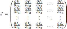
given a vector field f : Rn 7→ Rn with (Cartesian) components
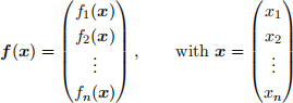
i.e., where each component of f , fi, is a function of the n co-ordinates x1,x2,x3,...,xn. Your function should have as inputs the function representing the vector field f and the point at which the Jacobean is to be evaluated x = x0 .
The function can use whatever finite-difference approximation that you feel is appropriate, and you are free to decide on the meaning of ‘reasonable’; you should explain the reasons for your choices in your answer. Ideally, your function should work for vector fields with any dimension n, and should select an appropriate finite-difference offset h automatically, but solutions for specific values of n or with h as an input are acceptable (though will receive lower credit). You should also ensure that your code is comprehensible to a user, and that the format of the inputs and outputs is clearly specified.
Use your function to calculate a numerical approximation to the Jacobian matrix, for the following vector fields:
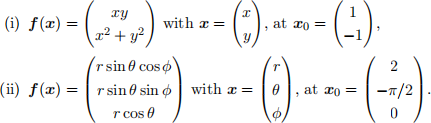
(6 marks)
Question 3: Numerical solution of ODEs
(a) (i) Write a Matlab function that uses the forward Euler method
to numerically solve the ODE system
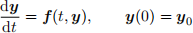
given a right-hand-side vector function f, initial condition y0, timespan [t0,tf] and number of steps N, where h = (b − a)/N. You may wish to use the file myEuler.m on Blackboard as a starting point.
(2 marks)
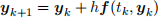
(ii) The iteration
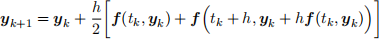
can also be used to solve the ODE system (2). Write a Matlab function, with the same inputs and outputs as above, that uses this method to solve the ODE system.
(2 marks)
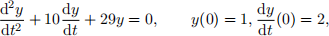
(b) Using your functions from part (a), solve the ODE
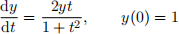
for t ∈ [0, 10], using the two methods in part (a), with stepsizes (i) h = 1, and (ii) h = 0.1. Plot graphs of the numerical and exact solutions of the ODE, as functions of time, and explain what they show.
(4 marks)
(c) Write a Matlab function that can find the global truncation error, E, between the exact solution y(t) and numerical solution y˜(t) of an ODE, measured as
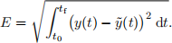
Use it to find the order of the global truncation error of the two methods in part (a), when used to solve the ODE in part (b), by plotting a graph of E against h for a suitably-chosen range of h. Which is the better method, and why?
(7 marks)
(d) Now use the two methods in part (a) to solve the ODE problem
for t ∈ [0, 10], with stepsizes (i) h = 1, and (ii) h = 0.1. Using ode45 to find the exact solution, plot graphs of the numerical and exact solutions of the ODE, as functions of time. Explain what is happening, and why.
(5 marks)
2021-12-03