Hello, dear friend, you can consult us at any time if you have any questions, add WeChat: daixieit

Miniproject – Numerical Linear Algebra – 3NMNLA4 – Resit

Background

I. Let Ω C R2 be an open, bounded domain with boundary Γ and consider the following  reaction-diffusion problem:

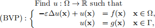
where ε > 0.  The finite element method (FEM) applied to (BVP) yields a linear system of equations of the form

Ku := (εA + M)u = f ,                                                               (1)

where A, M ∈ RN ×N are symmetric and positive-definite matrices. In particular,

•  A corresponds to a FEM discretisation of the negative Laplacian operator (-∆);

•  M represents a FEM discretisation of the identity operator  (it is in fact the mass matrix arising also in FEM discretisations of generalised eigenvalue problems).

•  The right hand side f ∈ RN  is related to the data f (x) and g(x).

Examples of matrices A,M , but also of right hand side vectors f can be generated using poisson2d .m for the case Ω = (0, 1)2 , f (x) = 1, g(x) = 0.

A related problem that will be referred to is the generalised eigenvalue problem

Awi = μiM wi.                                                                     (2)

II. We associate with (BVP) the following time-dependent (or initial value) problem:

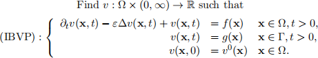
Note that if  lim t→∞ v(x, t) = v∞ (x), then v∞ (x) is called the steady-state solution of (IBVP).

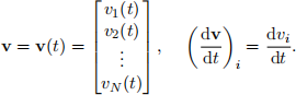
A certain FEM discretisation of (IBVP) yields the following system of initial value problems (IVP)

where, unlike the vector u in (1), the vector v has entries which depend on time:

III. Problem (3) is solved numerically by using finite difference approximations for the time derivative of v.  In the case of one-step methods, this results in recurrences of the form

V k+1 = V k + hΦk , V0 = v0 ,

where V k  ≈ v(tk) and where  {tk  = kh, k = 1, . . . , Nt} is  a discrete set of Nt  points  in time  (with  h > 0 the time-step). Different choices of Φ k  correspond to different methods.  For details, see Appendix B, Lecture notes.

Outline The aim of this miniproject is to work with the systems of equations (1) and (3) and use NLA to derive a set of theoretical and practical results. In the following, Q1 contains a set of results necessary in Q2, while Q3 suggests a certain practical approach and investigation via Matlab.

1. (a) Let C ∈ Rn×n  be a diagonalisable matrix with eigenvalues αi, i = 1, . . . , n. Let p,q be polynomials and assume that q(αi) ≠ 0 for all i = 1, . . . , n. Consider the generalised eigenvalue problem

p(C)vi = βiq(C)vi.

Show that βi  = p(αi)/q(αi) for i = 1, . . . , n.

(b) Let v0 , g ∈ Rn , G ∈ Rn×n  be given and consider the recurrence

v k+1 = Gv k + g.                                                              (4)

Show by induction that for all k ∈ N

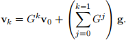
Deduce that

v k  = Gkv0 + (I - G)-1(I - Gk )g.

[15]

2. The system of initial value problems (3) can be given the general form

The Crank-Nicolson method with constant time-step h for system (3) is a two-term recurrence of the form

(a) Find F in terms of K, M and f. Hence, write recurrence (5) in the form (4), for a matrix G and vector g which you should specify.

(b) Let G denote the matrix found in part (a). Show that ρ(G) < 1 for all h > 0. [Hint: write the eigenvalue problem for G as a generalised eigenvalue problem and use the result from Q1(a) with C = M-1 K].

(c) Let u be the solution of linear system (1). Using the result from Q1(b), show that

Comment on this result, in view of problems (IBVP), (BVP) described above.                                    [15]

3. To implement efficiently recurrence (5), we re-write it in the form

where S is a sparse matrix which you should specify.

(a) Write a Matlab file cnmini .m to implement the Crank-Nicolson method in the form (6), using at every time step the preconditioned Steepest Descent method (PSD) with M as a preconditioner.  The input should be K, M, h, v0 , f , Nt  (in this exact order), while the output should be

•  a column vector v containing V Nt;

•  a column vector e containing the values Ⅱu - V kⅡ2 , (k = 1, . . . , Nt);

•  a column vector k containing the number of PSD iterations required at every time step in order to satisfy a fixed stopping criterion.

(b) By considering the generalised eigenvalue problem Swi  = λiM wi, find the eigenvalues of the precondi- tioned system in terms of ε, h and µi.

(c) By making suitable choices of parameters ε,h,N , describe an experiment that confirms the expected rate

of convergence of the algorithm from part (a) in the limit N → ∞, given the eigenvalue analysis from

part (b). Write a script file testcn .m to implement your experiment. Your script should display in the

command window and/or plot any relevant quantities that validate the statements you aim to verify in your experiment.       [20]

Notes on marking procedure for Q3(a) and Q3(c)

The following issues with the files eulermini .m,  testeuler .m may attract penalties:

• file does not use the suggested input and output as described in the question;

• file does not run due to incorrect syntax;

• file runs but output is incorrect;

• file does not contain the necessary local files, or the functions referenced are not in the uploaded zip file;

• implementation  does  not  follow  a  least  complexity  approach/principle  (e.g.,  generating  a  dense  matrix inverse in order to solve a linear system etc.);

• file does not suppress unnecessary output;

• file does not contain comments/descriptions;

• file is partially or entirely identical to other submitted files.