• This assignment is due Friday, February 16, 2024, at 11:55 pm.

• You must write your answers and R code using Rmarkdown (template provided with Assignment  1) and generate a single  PDF file. Submissions not generated by Rmarkdown will not be graded and receive zero marks.

• Submissions must be done via Gradescope. You must carefully assign questions to their corresponding pages. Submissions without questions assigned to pages will not be graded. Questions with no pages assigned to them will receive zero marks.

• Always show all your work and add comments to your code explaining what you are doing.

• Each student must submit their own work and use their own words to answer questions and explain results. The use of AI tools  (such as ChatGPT) to generate answers is prohibited. Scholastic offences are taken seriously, and students are directed to read the appropriate policy, specifically, the definition of what constitutes a Scholastic Offence, at the following Web site: http://www.uwo.ca/univsec/pdf/acade mic_policies/appeals/scholastic_discipline_undergrad.pdf

Question 1

a) Show that the deviance of a linear regression model (Gaussian responses) is the residual sum of squares (RSS).

b) Show that the deviance of a Poisson regression model can be written as

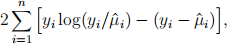
where µ(ˆ)i  = exp(xi(T)β(ˆ)).

Question 2

The dataset bacteria contains data on the presence of the bacteria H. influenzae in children with middle-ear infection in Australia after a certain treatment. The command ?bacteria can be used to check the description of each variable in the dataset.

suppressMessages(library(MASS))

suppressMessages(library(faraway))

bacteria$ap  <- factor(as.character(bacteria$ap),levels=c("p" , "a"), labels  = c ("Placebo" , "Active"))

a) Fit a logistic regression model to assess the association between the response variable y (presence or absence of bacteria) with ap, a covariate indicating treatment type (active treatment or placebo), and week.  Include in your model a term for the interaction between week and ap. Report the fitted model summary table.

b) Write the corresponding model equation for the model fitted in part a) showing the link

function and its relationship with the predictors.

c) Interpret the estimated coefficients in terms of odds.

d) Why using the p-values (based on z-values) provided in the summary table in a) may not be a good way of assessing the significance of individual predictors?  What are two other better strategies for doing such assessment?

Question 3

How does age affect male elephant mating patterns? An article by Poole (1989) investigated whether mating success in male elephants increases with age and whether there is a peak age for mating success. To address this question, the research team followed 41 elephants for one year and recorded their ages and number of matings. The data is found in elephant. csv, and the variables are:

• MATINGS = the number of matings in a given year

• AGE = the age of the elephant in years.

elephant  <- read.csv ("elephant. csv")

str (elephant)

##  ' data. frame ' :        41  obs .   of    2  variables:

##    $  AGE          :   num     27  28  28  28  28  29  29  29  29  29   .  .  .

##    $  MATINGS: num     0  1  1  1  3  0   0  0   2  2  .  .  .

a) Create a histogram of MATINGS. Is there preliminary evidence that number of matings could be modeled as a Poisson response? Explain.

b) Plot MATINGS by AGE. Add a least squares line.  Is there evidence that modeling mating counts using a linear regression with age might not be appropriate?  Explain. (Hints: fit a smoother; check residual plots).

c) For each age, calculate the mean number of matings.  Take the log of each mean and plot it by AGE.

i. What assumption can be assessed with this plot?

ii. Is there evidence of a quadratic trend in this plot?

d) Fit a Poisson regression model with a linear term for AGE. Interpret the coefficient for AGE.

e) Construct a 95% confidence interval (use the confint() function in R) for the slope and interpret it in context.

f) Based on the model fitted in part d), what is the predicted mating rate for a 31-year-old elephant? Using the results from part e), construct a 95% confidence interval for your prediction.

g) Are the number of matings significantly related to age? Test with a drop-in deviance test.

h) Add a quadratic term in AGE to determine whether there is a maximum age for the number of matings for elephants.  Is a quadratic model preferred to a linear model? To investigate this question, use a drop-in deviance test.

i) What can we say about the goodness-of-fit of the model with age as the sole predictor (no quadratic term)?

j) Fit a quasi-Poisson regression model with a linear term for AGE.

i. How do the estimated coefficients change?

ii. How do the standard errors change?

iii. What is the estimated dispersion parameter?

iv. An estimated dispersion parameter greater than 1 suggests overdispersion. When adjusting for overdispersion, are you more or less likely to obtain a significant result when testing coefficients? Why?

Question 4

The data set NMES1988 in the AER package contains a sample of individuals over 65 who are covered by Medicare in order to assess the demand for health care through physician office visits, outpatient visits, ER visits, hospital stays, etc. The data can be accessed by installing and loading the AER package and then running data(NMES1988).  More background information and references about the NMES1988 data can be found in help pages for the AER package.