ECE3093 semester 1 2024: Assignment 1
Hello, dear friend, you can consult us at any time if you have any questions, add WeChat: daixieit
ECE3093 semester 1 2024: Assignment 1
Instructions
Documentation:
. The assignment documentation consists of two parts, this .pdf ile and an associated .ipynb notebook.
. This ile contains background information and all of the assignment questions.
. The notebook contains some sample code and provides a template within which you can complete the code required for the assignment.
. Any additional iles required for the assignment will be available via Moodle.
While Python is encouraged, you may use Python or MATLAB to complete the assignment. If you use MATLAB, it will be your responsibility to appropriately translate the skeleton code given in Python to MATLAB for use.
Submission information:
. Please submit your assignment via Moodle by the due date listed in Moodle.
. Please submit:
– One .pdf ile with your answers to the questions.
– One code ile (either .ipynb or .m) with the code you have written for the assignment
Marking:
. The assignment will be marked out of 100 and contributes 15% to your inal mark for the unit
. The contribution of diferent questions to the total assignment mark is indicated next to each question.
. The weight assigned to tasks may not always relect their diiculty.
. Coding tasks will be marked based on a combination of clarity of the code and the approach you took to solve the problem.
. Questions that involve mathematics or explanations of your reasoning will be marked based on a combination of correctness of answers (if there are single correct answers) and clear logical reasoning demonstrating your understanding of relevant concepts.
. Tasks marked ‘C’ require you to write code in your code submission.
. Tasks marked ‘Q’ require you to give a written answer in your .pdf submission. (For some of these tasks you may wish to write additional code to aid your answer. Doing so is optional.)
1 Part 1: reconstruction and smoothing a noisy sampled signal
Consider an vector z 2 R1001 that is obtained by sampling a smooth signal of 1 second duration at equally spaced intervals of 0.001 seconds. The vector is indexed so that 从k corresponds to the signal value at time 0.001k for k = 0)1). . . )1000.
Now suppose that this vector z is downsampled by a factor of 50 via a noisy process. (Down- sampling means by a factor of 50 means keeping every 50th sample only.) This gives a new vector y 2 R21 deined by
g k = z50k + wk for k = 0)1). . . )20
where each 山k represents random additive noise.
In this part of the assignment you explore diferent ways to reconstruct an estimate x 2 R1001 of the unknown smooth signal z 2 R1001 from the downsampled noisy signal y 2 R21 .
1.1 Optimising a combination of data itting and smoothness (40 marks)
The irst approach is based on optimising the objective function

where > 0 is a parameter. Perform the following tasks and answer the associated questions.
C1 (5 marks) Write code that forms matrices C and D so that the optimisation problem (1) is equivalent to a problem of the form
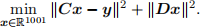
One of your matrices should depend on a parameter . Initially set = 0.01.
C2 (5 marks) Write code that forms a matrix P and a vector q so that the matrix equation Px = q represents the normal equations associated with the least squares problem (1).
Q1 (5 marks) Identify any notable properties that the matrix P appearing in the normal equations has. (Hint: you may wish to compute quantities related to the matrix P to help you answer this question.)
C3 (5 marks) Write code that applies an appropriate numerical method to solve the normal equations and ind the least squares estimate x.
Q2 (5 marks) Briely explain why you chose the method you did in C3 to solve the normal equations.
C4 (5 marks) Compute the least squares estimate x based on a QR decomposition of the matrix A. Check that your answer is consistent with the answer obtained in C3.
C5 (5 marks) Plot the original signal z, the noisy downsampled signal y, and the least squares estimate x on the same set of axes. Do this for = 0.01)1)100, giving three plots in total.
Q3 (5 marks) Briely discuss how the diferent values of the parameter afect both the denoising
and the reconstruction that is achieved.
1.2 Exactly interpolating the measurements (20 marks)
If the noise level is very small, it may be appropriate to compute an estimate x that exactly agrees with the downsampled signal and minimises a criterion that encourages the reconstructed signal x to be smooth, i.e.,

where D is the matrix you found in C1.
Q4 (4 marks) Explain how to apply a change of variables to (2) so that it can be reformulated as

In particular, explain how the variable w is related to the variable x, and how the matrix A and the vector b can be formed from the data vector y and the matrices C and D from C1.
C6 (4 marks) Using appropriate numerical methods, construct and solve (3) for w, and then solve the original problem (2) for x.
Q5 (4 marks) Explain why you chose the methods you did in C6.
C7 (4 marks) Plot the original signal z, the noisy downsampled signal y, and the solution of (2) on the same set of axes.
Q6 (4 marks) Explain how you can obtain the solution of (2) by taking an appropriate limiting value of in (1). Which method (solving (2) or solving (1) with a limiting value of ) would you recommend? Why?
2 Part 2: illing in missing pixels in an image
Consider an m n greyscale image, represented via an m n matrix X with each entry taking values between 0 (black) and 1 (white). Consider a situation where a collection of pixels are missing or occluded. One context where this can arise is if there are objects covering parts of the image. Here we will focus on situations where the pixels are missing at random.
In this part of the assignment we will look at some simple methods of inpainting, where we try to ill in the part of the image that has been lost when pixel values are missing.
In part 1 we used smoothness as additional information to help reconstruct a signal from partial measurements, here we will focus on using the fact that many natural images are approximately low rank to help with image reconstruction.
In the accompanying notebook, you are given code that:
. Loads an image, converts it to greyscale, and converts it to an array X.
. Generates a boolean array indicating which pixels are measured (with value True) and occluded (with value False).
. Generates an occluded version of the image where the occluded pixels are set to zero, and stores it in an array Y.
Before running the code, you will need to download the ile ece3093assignmentpic.png from Moodle and upload it into your Google drive. Then the notebook can load the image from your drive. You may need to modify the path in the code given so that it points to where you choose to save this image. If you would like to experiment with other images apart from this one, feel free to do so!
We will make use of logical indexing for numpy arrays in some parts of the assignment. You may need to learn the basics of how this works if you haven’t come across it before.
2.1 Building a chequerboard image (10 marks)
In this section, you will write code to build a 500 pixel by 500 pixel image where each pixel is either black (value 0) or white (value 1) and where the black and white pixels form a chequerboard pattern, consisting of a 10 10 grid with each square alternating between being a 50 pixel by 50 pixel black square or a 50 pixel by 50 pixel white square.
C8 (3 marks) Write code to form the chequerboard image described above and store it in an array Xch. Also form the occluded image Ych.
Q7 (3 marks) What is the rank of the matrix Xch you have constructed that represents the chequerboard? What are its singular values?
Q8 (4 marks) If the chequerboard were a pa qa pixel image made up of a p q grid consisting of a-pixel by a-pixel alternating black and white squares, what would be the singular values of the matrix associated with this general chequerbaord image? Explain your answer.
2.2 Inpainting by low rank approximation (10 marks)
In this section, you implement a very simple (and not very efective) inpainting method. You will take the occluded version of an image, stored in the matrix Y , and ind a best rank r approximation. In other words, you will solve

C9 (4 marks) Write code to ind the best rank r approximation to Y (the occluded version of the image).
C10 (3 marks) Run this code for the occluded chequerboard image Ych and the loaded occluded image Y, and for various values of r, and display a selection of the resulting image reconstruc- tions.
Q9 (3 marks) Briely discuss how the parameter r afects the image reconstruction in each case.
2.3 Inpainting by alternating low-rank approximation and data itting (20 marks)
The method of inpainting by simply taking a low-rank approximation is clearly not very successful! A basic problem with the method is that it generates images that have the wrong pixel values for pixels where we know the correct values. A simple ix to this problem is to consider an alternating scheme where we use the best rank r approximation of the whole image to determine new values for the missing pixels, and only update the values of the missing pixels.
. Input: occluded image array Y and rank parameter r
. For k = 0, 1, . . . , K:
– Compute Yr, the best rank r approximation of Y via (4)
– Update Y by setting Yij = [Yr]ij where (i, j) range over the occluded pixels
C11 (8 marks) Write code to implement the alternating scheme described above. You will need to decide on some maximum number of iterations for the loop (you optionally want to implement a stopping criterion that stops if you detect that the scheme has converged).
C12 (5 marks) Run this code for the occluded chequerboard image Ych and the occluded loaded image Y, and for various rank parameters r and numbers of iterations K. Display a selection of the resulting image reconstructions.
Q10 (7 marks) Briely compare the reconstructions achieved herewith the reconstructions from C9. For which image does the reconstruction work the best? Why do you think this is the case? Discuss how the parameter r afects the image reconstructions.
2024-04-13