Math Application Project #3: Bézier Curves
Hello, dear friend, you can consult us at any time if you have any questions, add WeChat: daixieit
Math Application Project #3: Bézier Curves
due Sunday April 14, 2024 by 11:59 PM
We have learned about cubic spline interpolation. Here you will work with Bézier curves, another kind of spline which are essential for computer aided-design, manufacturing, and digital animation.
Bézier curves are splines that allow the user to control the slopes at the knots. In return for the extra freedom, the smoothness of the first and second derivatives across the knot, which were main features of the cubic splines we derived in class, are no longer guaranteed. Bézier splines are appropriate for cases where corners (discontinuous first derivatives) and abrupt changes in curvature (discontinuous second derivatives) are occasionally needed.
Pierre Bézier developed the idea during his work for the Renault automobile company. The same idea was discovered independently by Paul de Casteljau, working for Citroen, a rival automobile company. It was considered an industrial secret by both companies, and the fact that both had developed the idea came to light only after Bézier published his research.
Theory: Equations for Bézier Curves
Each piece of a planar Bézier spline is determined by endpoints of the spline curve (x1 , y1) , (x4 , y4 ) and control points (x2 , y2) , (x3 , y3 ) as shown in the Figure below. The curve leaves (x1 , y1 ) along the tangent direction (x2 − x1, y2 − y1 ) and ends at (x4 , y4) along the tangent direction (x4 − x3 , y4 − y3 ). The equations that accomplish this are expressed as a parametric curve (x(t), y(t)) for 0 ≤ t ≤ 1 .
We could show that the equations below represent Bézier curves. You will not do that for this project. Rather, you will assume these equations are correct and will write code to implement them.
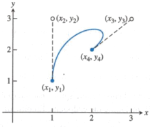
Figure 1.
Given endpoints (x1 , y1 ), (x4 , y4 ) and control points (x2 , y2 ), (x3 , y3 ), let
bx = 3(x2 − x1 )
cx = 3(x3 − x2 ) − bx
dx = x4 − x1 − bx − cx
by = 3(y2 − y1)
cy = 3(y3 − y2) − by
dy = y4 − y1 − by − cy .
Then the Bézier curve is defined for 0 ≤ t ≤ 1 by
x(t) = x1 + bxt + cxt2 + dxt3
y(t) = y1 + byt + cyt2 + dyt3 .
We could show that these equations lead to x(0) = x1 , x(1) = x4 , x′ (1) = 3(x4 − x3 ), and that analogous facts hold for y(t).
Your Programming Assignment: Drawing Bézier Curves
Here you will explore how to use Bézier curves to draw letters and related shapes. They can be implemented by writing MATLAB code that creates its own PostScript file. You may work with a partner for this project.
PostScript fonts are built directly from Bézier curves. Here is a complete PostScript file that illustrates the curve shown in Figure 1. You can also find this file inside the Project 3 .zip file as beziersample.ps.
%!PS
newpath
100 100 moveto
100 300 300 300 200 200 curveto
stroke
The first line identifies the file as a PostScript file. The newpath command initiates the curve. PostScript uses a stackand postfixnotation. The moveto command sets the current plot point to be the (x, y) point specified by the last two numbers on the stack—in this case, the point (100,100). The curveto command accepts three (x, y) points from the current stack and constructs the Bézierspline starting at the current plot point, treating the three (x, y) pairs as the two control points and the endpoint, respectively. The stroke command draws the curve. If the preceding file is sent to a PostScript printer (for example, double-clicking on the file on my Mac opens the file with Adobe Distiller), the Bézier curve of Figure 1 will be printed. The coordinates have been multiplied by 100 to match the conventions of PostScript, which are 72 units to the inch. A sheet of letter-sized paper is 612 PostScript units wide and 792 high.
PostScript fonts are drawn on computer screens and printers, using the Bézier curves of the curveto command. The fill command will fill in the outline if the figure is closed.
For example, the upper case T character in the Times Roman font is constructed out of the following 16 Bézier curves (each line consists of the numbers x1 y1 x2 y2 x3 y3 x4 y4 that define one piece of the Bézier spline. This data is also available as a text file , proj2_exercise2_letterT.txt):
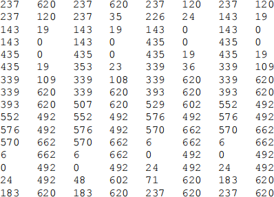
To write a PostScript file that writes the letter T, one needs to moveto the initial endpoint (237,620), add the next two control points and endpoint (237, 120), and follow with a curveto command. After that, the current position will be (237, 120), and the second curve is drawn by the command
237 35 226 24 143 19 curveto
Fourteen more curveto commands finish the letter T, as shown in Figure 2.
Here are your Programming & Design tasks:
1. Write a MATLAB function that reads in an n x 8 matrix of numbers from an input text file, each row representing the four control points of a Bézierspline. Your program should then output a file (ending in .ps) which can be opened by any standard PostScript reader and print the desired curves. Hint: the MATLAB functions dlmread, readmatrix, and readtable are easy to use.
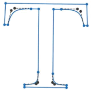
Figure 2. Times Roman T made with Bézier splines. Blue circles are spline endpoints, black circles are control points.
To test your code, reproduce the letter T from Figure 1 above by reading proj2_exercise2_letterT.txt. Then run your code on the two files, proj2_exercise2mysteryOne.txt and proj2_exercise2mysteryTwo.txt. What symbol does each of these ‘mystery’ files create? Include the answer in your live script.
2. Now write a MATLAB function that reads in a text file whose format matches the proj2*.txt files, but now prints the Bézier curves in a MATLAB figure. (That is, your MATLAB figure should look analogous to what you get from the .ps files from Exercise #1.) Use the parametric Bézier curve equations defined above. The axis square command may be useful here, to give your figure a nice aspect ratio.
3. Consider the shield from F&M Diplomats logo below. Use your Bézier curve plotting function to create a MATLAB figure which reproduces the outline of the shield and the ‘shiny reflection ’ as accurately as you can. Estimate the endpoints and control points of each Bézier curve by hand; be ready to revise them later as needed to improve your result. You can either keep the shield as two separate pieces, or connect them as in the example shown Appendix 1. Gridlines have been added to the logo below for reference. Submit the endpoints and control points as a single .txt file where each line includes the endpoints and control points of a Bézier curve, consistent with the proj2*.txt files above. Also submit a marked-up printout/screenshot of the Diplomats logo, which shows evidence of your work.
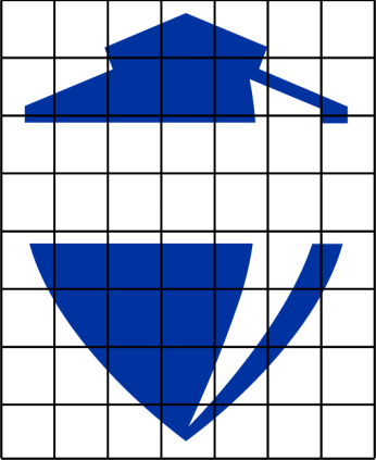
Figure 3. Here is the F&M shield you will reproduce for #3.
Notes about your submission:
Your files for the Programming Tasks (.m files,.txt file and labeled sketch showing your work for #3) should be submitted as a compressed .zip archive on Canvas.
2024-04-11