Project 2
Hello, dear friend, you can consult us at any time if you have any questions, add WeChat: daixieit
Project 2
Two main template files are available; modify these but keep their names:
• A template RMarkdown document, report.Rmd, that you should expand with your answers and solutions for this project assignment,
• A template code.R file where you should place function definitions needed by report.Rmd, with associated documentation.
Instructions:
• Include your name and student number in both report.Rmd and code.R.
• Code that displays results (e.g., as tables or figures) must be placed as code chunks in report.Rmd.
• Code chunks that load the function definitions from code.R are included in report.Rmd (your own function definitions).
• You must upload the following three files as part of this assignment: code.R, report.Rmd and a generated html version of the report with the file name report.html and you you will be marked based on the report.html file.
• Appendix code chunks display the code from code.R without running it.
• Use the styler package Addin for restyling code for better and consistent readability works for both .R and .Rmd files.
• Use echo=TRUE for analysis code chunks and echo=FALSE for table display and plot-generating code chunks.
• The main text in your report should be a coherent presentation of theory and discussion of methods and results, showing code chunks that perform computations and analysis.
The project will be marked between 0 and 40, using the marking guide CWmarking posted on Learn.
Submission should be done through Gradescope.
Part 1: 3D printer
Here, you will use the filament1 dataset from Project 1, which contains information about a 3D printer that uses rolls of filament that get heated and squeezed through a moving nozzle, gradually building objects. The objects are designed using a CAD program (Computer Aided Design) that estimates how much material will be required to print them. The data file "filament1.rda" contains information about one 3D-printed object per row. The columns are
• Index: an observation index
• Date: printing dates
• Material: the printing material, identified by its colour
• CAD_Weight: the object weight (in grams) that the CAD software calculated
• Actual_Weight: the actual weight of the object (in grams) after printing
Consider two linear models, A and B, for capturing the relationship between CAD_Weight and Actual_Weight. Denote the CAD_weight for observation i xi , and the corresponding Actual_Weight yi . As in Project 1, the two models are defined by
• Model A: yi ∼ Normal[β1 + β2xi , exp(β3 + β4xi)]
• Model B: yi ∼ Normal[β1 + β2xi , exp(β3) + exp(β4)x2i]
Recall that in Project 1, you built functions to estimate the parameters from Models A and B. In exercises 1-5 described below, you will build predictive distributions for models A and B and access the performance of both models to predict new data.
1. Create a function filament1_predict with similar behavior to the R built in lm.predict that computes predictive distributions and 95% prediction intervals for a new dataset. Your function should return a data.frame with variables mean, sd, lwr, and upr, summarizing the predictive distribution for each row of the new data. The function filament1_aux_EV in code.R evaluates the expectation and variance for model A and B and can be used to help constructing the predictive distributions in filament1_predict. The arguments theta and Sigma_theta needed in filament1_aux_EV can be obtained by first estimating models A and B using the filament1_estimate and neg_log_lik functions in code.R to retrieve the estimated expected value and variance for each model (recall from Project 1). Next, use your function to compute probabilistic predictions of Actual_Weight using the two estimated models and the filament1 as new data. Use a level of significance of 5% for computing the prediction intervals. Note that in this exercise, the data for estimating and predicting the models are the same. Inspect the predictions visually.
2. Write functions to evaluate the squared error (ES) and Dawid-Sebastiani (DS) scores.
3. Here, you will use the functions created in the previous exercises to perform leave-one-out cross-validation. Implement a function leave1out that performs leave-one-out cross-validation for the selected model for each observation i = 1, . . . , N. In this function, you should first estimate the model parameters using {(xj , yj ), j = i}, compute the prediction information based on xi for prediction model Fi , and then compute the required scores S(Fi , yi). The output should be a data.frame that extends the original data frame with four additional columns mean, sd, se and ds of leave-one-out prediction means, standard deviations, and prediction scores. Use leave1out to obtain average leave-one-out scores S(Fi , yi) for each model and type of score for filament1 data. Present the results and interpret them.
4. Construct a Monte Carlo estimate of the p-value to test the exchangeability between model predictions from A and B against the alternative hypothesis that B is better than A. Compute Monte Carlo standard errors, draw conclusions, and investigate whether one model is better at predicting than the other.
Part 2: Archaeology in the Baltic sea
In 1361, the Danish king Valdemar Atterdag conquered Gotland. A plunder of Visby followed the conquest. Most of the defenders (primarily local farmers who could not take shelter inside the city walls) were killed in the attack and were buried in a field outside of the walls of Visby. In the 1920s, the gravesite was subject to several archaeological excavations. A total of 493 femurs (256 left and 237 right) were found. One question that arises is the number of people that were buried at the gravesite. It must reasonably have been at least 256, but how many more?
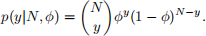
To build a simple model for this problem, assume that the number of left (y1 = 256) and right (y2 = 237) femur are two independent observations from a Bin(N, ϕ) distribution. Here N is the total number of people buried and ϕ is the probability of finding a femur, left or right, and both N and ϕ are unknown parameters. The probability function for a single observation y ∼ Bin(N, ϕ) is
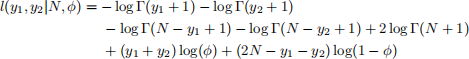
The combined log-likelihood l(y1, y2|N, ϕ) = log p(y1, y2|N, ϕ) for the data set {y1, y2} is then given by
Before the excavation took place, the archaeologist believed that around 1000 individuals were buried, and that they would find around half on the femurs. To encode that belief in the Bayesian analysis, set ξ = 1/(1+ 1000), which corresponds to an expected total count of 1000, and a = b = 2, which makes ϕ more likely to be close to 1/2 than to 0 or 1.
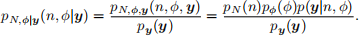
The posterior probability function for (N, ϕ|y) is
Let N have a Geom(ξ), ξ > 0, prior distribution, and let ϕ have a Beta(a, b), a, b > 0, prior distribution:
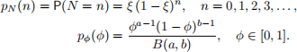
Monte Carlo integration can be used to estimate the posterior expectations of N and ϕ. Consider prior distributions N ∼ Geom(ξ), 0 < ξ < 1, and ϕ ∼ Beta(a, b), a, b > 0. Furthermore, consider the prior distributions as sampling distributions for the Monte Carlo integration, such that samples n [k] ∼ Geom(ξ) and ϕ [k] ∼ Beta(a, b), cand be used to compute Monte Carlo estimates:
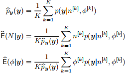
1. Write a function arch_loglike that evaluates the combined log-likelihood log[p(y|N, ϕ)] for a collection y of y-observations. If a data.frame with columns N and phi is provided, the log-likelihood for each row-pair (N, ϕ) shoule be returned.
2. Write a function estimate that takes inputs y, xi, a, b, and K and implements the above Monte Carlo integration method to approximate py(y), E(N|y), and E(ϕ|y). Test the function by running estimate(y=c(237,256), xi=1/1001, a=0.5, b=0.5, K=10000) and comment on the results.
2024-04-08