MA416 - Analysis of Variance - Mini-Exam 2

Directions (Please Read) : The time permitted for this exam is 40 minutes. You must show all work to receive full, if any, credit (where applicable). A basic scientific or TI calculator may be used, in addition to a 3” x 5” note card (handwritten, back and front); no notes, books, search engine, cell phone, any other person, device, or resource aside from yourself can be used to get assistance on any portion of this exam. Failure to adhere to any of these (or university) policies will result in a zero for this assessment. Please try to adhere to the recommended time limits on each question block.

[2 mins] For the following (1) – (4), circle either “True” or “False” regarding the validity of the entire statement provided.

1.    True        False       The null hypothesis for a Kolmogorov-Smirnov test and a Lilliefors’ testis the same.

4.    True         False       You can always fit a linear model onto a bivariate data set.

[15 mins] For the following (5) – (7), suppose you have the following datasets, and you want to test whether or not they have the same medians (or not). You datasets are shown below. Do not use any software to assist you.

S1   = {5, 2, 8, 7, 8}     S2   = {8, 7, 4, 1, 9, 2}

5.     Here n1   = 5 and n2   = 6 .  Complete  the  following  table  by  providing  the  global  ranks  for  each  element,  with  average convention defining ranks for tied values.

6.    Calculate the average ranks for the mentioned samples below. Place your final answer in the table, and justify all work below it to support your answers.

7.    Calculate the  associated  Mann-Whitney test  statistic for this test. Show work to support your answer.  Denote your final answer in the form (MW)stat   = ⋯ .

8.     [5 mins] Suppose we are working with the following null and alternative hypotheses.

H0 : Populations A and B are heteroscedastic to one another

Ha : Populations A and B are homoscedastic to one another

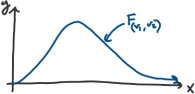
Suppose we define a test statistic by Below is a sketch of an F distribution. Shade in the area that would be approximately equal to the probability of committing a Type I error. Shade completely so your shaded region is obvious.

[20 mins] For the following (9) - (12), suppose you collect abivariate data set that has the following characteristics, where A and B are your variables.

9.    Suppose that you want to  use variable A to  predict variable B. What  is the associated slope for your  least squares  linear regression line? Show work to justify your answer.

10.  Suppose you want to use variable B to predict variable A. What is the associated slope for your least squares linear regression line? Show work to justify your answer.

11.  Suppose that you want to use variable B to predict variable A, and you have a B value of 43.2. What would be your associated predicted value of A? Show work to justify your answer.

12.  Suppose that you want to use variable B to predict variable A. What is the associated mean square error for your residuals equal to? Show work to justify your answer.