MATH3001 project: Using Random Numbers to Solve Problems in Mathematics, Physics and Finance 2023/24
Hello, dear friend, you can consult us at any time if you have any questions, add WeChat: daixieit
MATH3001 project: Using Random Numbers to
Solve Problems in Mathematics, Physics and Finance
2023/24
Prerequisites:
MATH1715, MATH1725, some programming experience in a computer language like Python or R.
Preamble
During this project you will get a taste of doing original mathematical research. This involves being proactive in planning your project and finding ways to make things work. You will work partly in a team but mostly independently, to produce a group presentation and an individual report on your project.
We will begin by studying some topics together, and discussing some introductory homework tasks to gain experience of the topics. Later (for perhaps the last 60% of the project), each person will choose a different topic from the list in section 5 to investigate in greater depth, or may propose another topic to their supervisor.
All projects will require some investigation of the background theory, and some computational investigation of specific problems, but the balance between these is up to you. Your report will present all of your investigations, both the introductory ones and the more substantial one, explaining the background, results and conclusions in a style similar to that of a textbook, so that they could be understood by a maths undergraduate not familiar with the project.
1 Introduction to Monte Carlo methods
Most computer programming languages have a command which allows the user to generate random, or pseudorandom, numbers. For example, the “Python” language has a set of standard commands for generating random numbers (either integers or real numbers) from a wide range of standard distributions, such as the uniform and normal distributions [1]. The aim of this project is to investigate computational methods, known as Monte Carlo methods, which can solve a variety of mathematical and physical problems, to arbitrary accuracy, by using random numbers.
Random numbers can be used for statistical sampling (also called “Monte Carlo sampling”). A common application of this is in numerical integration, in which the function to be integrated is sampled at random points within the domain of integra- tion, in order to estimate the value of the integral [2, 3]. For integration in one dimen- sion, other numerical integration methods (such as Simpson’s rule) are usually more efficient than Monte Carlo Methods. But for multidimensional integrals, Monte Carlo methods become competitive, and for very large numbers of dimensions these are the only practical method for numerical integration.
Homework task 1:
The following are to be completed before the second supervised meeting. Please create presentable results that you can share on your screen (or upload to the TEAMs channel) for the second meeting.
You may choose to work in any standard programming language to which you have access, such as Python, R, C or Java. During the supervised sessions we will study examples in Python.
. Preparation. You should begin by making sure that you can edit a program file and execute the program (after first compiling it, if you are using a compiled lan- guage). Information on how to obtain Python has been sent by email. The best solution is to install a suitable programming language on your own computer. For Python we recommend installing the anaconda package which includes the integrated development environment (IDE) “Spyder”. “R Studio” provides a sim- ilar functionality for R if you prefer to use that.
. When learning a programming language or using an IDE for the first time, it is traditional to begin by writing a program to output the text “Hello World”. Make sure that you can do so. (This task is too simple to be included in the final report.)
. Run the Python code provided in the session (or your own version of it in your chosen programming language) to evaluate the mean and variance of a random sample drawn from the probability distribution(s) discussed in class. Then adapt the code to investigate different parameters and/or distributions as discussed. Check that the results make sense to you. If they do not, it may indicate a bug in the program. Edit the program until you understand what is happening.
. For your report and presentation you will need to be able to present your re- sults in the form of graphs and figures. In Python there is an extensive library of graphing functions called Matplotlib. One of the example Python codes uses this to plot a histogram of sampling from a uniform distribution, but this pack- age can do many other types of plots (for more examples and tutorials go to https://matplotlib.org). Create a figure or figures to show how the number of samples affects the accuracy of capturing a distribution.
2 Monte Carlo Integration
A good reference for this section is chapter 7.7 of Ref. [4], which is available online at http://numerical.recipes/book/book.html or there are print copies in the library.
A common task in mathematics is the evaluation of integrals. Although in the problems set in undergraduate mathematics courses integrals can be performed an- alytically, this is rarely true in applications. Consequently we need numerical methods to approximate integrals as sums, so that
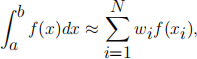
where we take a weighted sum of the values of the function at N points xi. In tradi- tional quadrature schemes such as the trapezium and Simpson’s rules [4] the posi- tions of the points are predetermined, e.g. equally spaced points.
However, in Monte Carlo integration the points are chosen randomly from a distri- bution. Since the mean value off can bedefined as
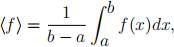
we can determine the value of the integral by sampling f to find its mean value. Thus if we draw N points, x1, . . . xN from a uniform distribution in the interval [a, b] then we can estimate the integral as,

Furthermore we can also estimate the error, by taking the square root of the mean squared error as

where σ2 is the variance of f over the interval. This means that the accuracy of the estimate improves as the square root of the number of points sampled.
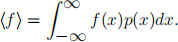
More generally if points are chosen from a probability distribution p(x) then
Homework task 2: For a general function f (x) obtain a formula for σ and hence an error estimate. How does this compare with quadrature schemes such as the
trapezium rule or Simpson’s rule? Write a program to estimate 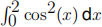 dx using
Monte-Carlo sampling. Compare the answer with a classical method such as the trapezium and Simpson’s rule. Is Monte-Carlo sampling a good way to estimate this integral?
2.1 Multi-dimensional Integration
The above example shows that there are better ways of integrating in one-dimension than Monte-Carlo (MC) methods. However, we shall discover that in multi-dimensional integration MC methods have their advantages.
Suppose we now consider the integration of the function f (x) over a D-dimensional domain x 2 V. As shown in the vector calculus course this can be computed via nested one-dimensional integrals as
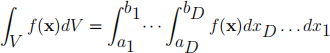
where V is contained in the hypercuboid (a, b) and we define f to be zero for points outside V. If we use a quadrature scheme with n points for each of the integrals we require a total of N = nD function evaluations. Now unless V fits precisely to the boundaries of the domain, f will be discontinuous. This means the error in each quadrature integral will scale as 1/n (since the higher order convergence of the trapezium and Simpson’s rules depend on function having continuous derivatives). Thus the total error will scale as N — 1/D. So when D is large the convergence is very slow. Even where we have a rectangular domain over which the function is differ- entiable the convergence rate we decrease as the number of dimensions increases. This is the “curse of dimensionality” .
Now suppose we use Monte-Carlo sampling. The integral can be estimated as

Hence the error scales as N-1/2 irrespective of the number of dimensions.
Homework task 3:
As an example let us consider calculating the area of the unit circle by integrating the function
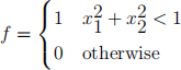
over the domain V = f(x1, x2) : jx1j < 1, jx2j < 1g. The answer is of course π. Write and execute your own program to estimate the integral using Monte-Carlo sampling. By plotting a graph, examine how the error changes with N. Run repeated calcula- tions for particular values of N and compare the variance with the error estimator.
How many samples would you need to calculate π to 3, 5 and 10 decimal places?
As usual, present your program and results at the next supervised meeting.
Extension task i:
Modify your programme to calculate the volume of a unit sphere and higher dimen- sional hyperspheres. The analytical formulas for the answers are given at http://thinkzone.wlonk. com/MathFun/Dimens.htm. How does increasing the dimension modify the convergence?
Extension task ii:
Examine what happens if you replace f with the function
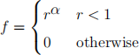
where 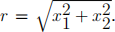 In particular look at what happens for the cases -2 < α < 0
when the integrand is singular at (0, 0) but integral remains convergent. Also see what happens at α = -2 when the integral has a logarithmic divergence.
3 The Metropolis-Hastings Monte Carlo Method
As we have seen, Monte Carlo sampling is particularly useful when the domain of interest is high-dimensional, so that it would take too long to visit every small element within it. One important application is to a branch of physics known as Statistical Mechanics.
Statistical Mechanics was developed to study the collective behaviour of vast num- bers of molecules. In that collective behaviour, particles exchange energy, leading to thermodynamic phenomena such as the freezing and boiling of water. A formalism was developed by the physicist Ludwig Boltzmann, for exact calculation of the large- scale behaviour (e.g. freezing or boiling) of a vast collection of particles (e.g. water molecules). Boltzmann’s method requires a particular function (related to the energy of the system) to be integrated over a very high-dimensional domain: the entire set of particles’ coordinates. That’s three coordinates for each of the N particles, leading to a 3N-dimensional domain, where N is of order 1023 in a typical sample such as a cup of water. It would take prohibitively long to explore such a domain thoroughly, in any numerical integration scheme. Instead, Monte Carlo methods are used to col- lect a representative sample of values of the integrand for a random set of particle positions.
However, the direct Monte Carlo method described in the previous chapters doesn’t work well for these applications because there isn’t a convenient way to select ran- dom samples from the target distribution. Instead we can use an indirect approach that exploits Markov chains to obtain a sequence of samples from a given distribu- tion, such methods are referred to as Markov Chain Monte Carlo methods or MCMC for short. A specific MCMC method developed to deal with the particular problems encountered in modelling physical materials is the “Metropolis Monte Carlo” scheme [5, 6], which we shall study in detail. The Metropolis algorithm was developed to sample microstates of systems in which the probability of states is given by the Boltz- mann distribution. It was later generalised by Hastings for more general probability distributions.
3.1 The Boltzmann distribution
Let us consider a system such as a material made up of interacting atoms, where the position of each atom can vary in space. We define a microstate of the system as the configuration defined by the positions of the atoms. For example, if the “system” is a single particle moving in one dimension then each microstate is defined by a coordinate x corresponding to the position of the particle. If the system is a set of N particles, then each microstate is represented by the set of vectors giving the particle positions, (x1 ; x2 ; : : : xN).
A key result from statistical mechanics is that the probability pi of finding a physical system in a given microstate i is given (subject to some conditions) by

where Ei is the energy of state i, T is the absolute temperature (usually measured in Kelvin: T = 273 + TC where TC is the temperature in Celsius) and kB is a constant known as Boltzmann’s constant ( kB = 1.38 根 10-23JK-1 in standard units). The product kBT is the typical thermal energy associated with a degree of freedom. The constant A is chosen so that the sum of the probabilities adds up to one.
For example, for a single thermal particle moving in one-dimension against a spring with spring constant , the energy E(x) is given by

so that the probability density p(x) at position x is given by,

![]() where in this case the normalisation constant is
where in this case the normalisation constant is 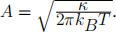
3.2 Metropolis-Hastings algorithm
To illustrate Metropolis-Hastings algorithm we consider the above example of a parti-
cle moving in one dimension against a spring. The sample code metropolisquadgraph. py runs the Metropolis-Hastings algorithm for this example.
Here is how the Metropolis-Hastings algorithm is implemented.
1. You need some way of storing the “state” of the state of the system on the computer - for example if you were simulating a collection of atoms, you would store the positions of all the atoms in computer memory. You also need to be able to evaluate the energy of the system depending upon the current state. In the code metropolisquadgraph. py , the state is just stored as the position, x, of the particle.
2. Start the system in a suitable microstate (i). In the code we choose x = 0.
3. Pick a random change from the current microstate (i) to another one (j). In our example, this is a shift in the position of particle from its current position xi to a new position xj= xi+ XΔx, where X is a random number drawn from the uniform distribution in the interval [-1, 1], and Δx is a step-length.
4. Calculate the ratio of probabilitiesrijbetween this new statej and the cur- rent state i,i.e. rij= p(xj)/p(xi). In the case of the Boltzmann distribution,
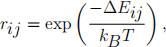
where ΔEij = Ej - Ej is the change in energy in moving from state i to state j.
5. Decide whether to accept the change of state. If the ratio rij ≥ 1, i.e. ΔEij 0 meaning that we are moving to a lower energy then we always ac- cept the change of state. But if rij < 1 meaning that energy increases, i.e. ΔEij> 0, we accept the change of state only with probability rij.
In practice, the way to achieve this is to generate a random numbers uniformly distributed between 0 and 1. If s < rij then accept the change of state, other- wise, discard the new state j and keep the old state i. In the Python programme metropolisquadgraph. py, you can see how these decisions are made with “if” statements.
6. Repeat (i.e. loop) steps 3-5 for as long as you need to. In the sample code, there is an outer loop which achieves this.
The algorithm generates a Markov chain with transition probabilities determined in step 5, and subject to some conditions (see below), over time the probability of finding the system in a given state should converge to the probability distribution, which for our example is given by equation (6).
This means that, for example, to estimate the average of some quantity f we can simply evaluate:

where the sum over i is a sum over a set of states reached after step 5 in the algorithm is completed and N is the number of states reached. Note that we include states in the sum irrespective of whether the last random change of state was successful,i.e. if the algorithm gets “stuck” in a given state for several times around the loop, then that state is counted multiple times in the sum because (presumably) it is a more likely state than some of the others.
The efficiency of the Metropolis-Hastings algorithm is due to the following rea- sons. First, the only information we need to know about the probability distribution is the relative probabilities of the states i and j, which in the case of the Boltzmann distribution can be found from the difference in the energies of the two states. For a complex multiparticle system this is much easier to find than the whole distribution function. Second, the algorithm naturally samples more from more probable states, which is a form “importance sampling” .
A few terms and conditions:
. If the initial state chosen in step 2 is not very likely then it can take the algorithm some time to settledown into sampling a reasonable set of microstates. If this is the case, it is sensible to run the algorithm through a number of loops to allow it to “equilibrate” before starting to calculate averages using (7), i.e. we discard a certain number of states reached during the first loops. How many times around the loop you need toequilibrate depends on the system, and the choice of random steps.
. For the “random change” in step 3, it must be the case that the probability of choosing a random move to state j from state i is exactly equal to the probability of choosing a random move from state j back to state i. This must be true for ALL pairs of states. Otherwise, a bias is introduced into the algorithm.
. The efficiency of the algorithm depends very much on how the “random changes” are made, which in the case of our example is governed by the choice of the step-size, Δx. If Δx is too small, then lots of moves will be accepted but the system doesn’t change much even after many loops of the algorithm. The sys- tem might get stuck in a local energy minimum but not have chance to explore all of the available configurations. However, if Δx is too large, there is a risk of not many changes being accepted.
. The “random changes” must allow the system the chance of exploring all pos- sibleconfigurations (the term for this is it needs to beergodic).
Homework task 4: Literature search
Find the original “Metropolis et al” paper which describes the algorithm.
Homework task 5: Theory
Can you show why the algorithm works? Explanations are available online or in books (and in the original paper by Metropolis et al). (If you have studied Markov Chain theory you should have the tools to do this, if you assume that ergodic prop- erty is satisfied). You need to consider the idea of detailed balance. The probability that a given loop through the algorithm takes you from state i to state j is the prob- ability pi of starting in state i, multiplied by the probability that a move from i to j is chosen, and that it is accepted. Similarly the probability that a given loop through the algorithm takes you from state j to state i is the probability pj of starting in state j , multiplied by the probability that a move from j to i is chosen, and that it is accepted. At “equilibrium” these two probabilities must be equal. have studied Markov Chain theory
Homework task 6: Simulation
The code metropolisquadgraph. py is a simple Python code implementing the Metropolis algorithm for a particle moving in one dimension with energy given by equation (5). It collects data for the frequency with which the particle visits various locations, and outputs data for a histogram of particle positions in a results file. Take a look at the code. See if you can see how it works. Have a play with the code - can you see what the effect of choosing large or small step size is? Set up the code so that it measures the average position of the particle? Measure the variance in particle position? Try a different energy profile - does the code still give the correct probability distribution? Can you break the algorithm - can you come up with a combination of a energy profile and a step size which means that parts of the energy profile are not visited (e.g. what if there is a large energy barrier between two minima)?
2024-04-02