Power Engineering Electromagnetics ‐ EEE349/EEE350 (2023‐2024)
Hello, dear friend, you can consult us at any time if you have any questions, add WeChat: daixieit
Power Engineering Electromagnetics ‐ EEE349/EEE350 (2023‐2024)
EEE349/EEE350 – Sem1 ‐ Assignment
Introduction
‐ This assignment depends on Sem 1 material.
‐ The assessment will be based on FEMM4.2 software
‐ The assignment might contain elements that have not been covered in the lectures. ‐ You should provide all workings and explanations in your solutions. Also, justify your
design selection, if any. These will variously count towards achieving full marks in this assessment.
‐ The FEMM4.2 material is not examinable in either TA or GA examinations.
‐ For individual values of the problem parameters, If you see the letter 'm' in red in the question or figures, this represents the last digit of your ID number. For example, if your ID number is
So, you will substitute every 'm' with the number 7.
If the last digit in your ID number is '0', you will substitute the 'm' number with 10.
Submission Details
You can complete your answers as a word‐processed document or as handwritten sheets (The word document is preferred). Please save or scan these respectively into a pdf file. Copy any graphs into a word document, then save them into a pdf file. Also, copy any figures or graphs from FEMM4.2 into a word document. As this submission is considered a formal report, The first‐page template is added to the same folder. Convert the first page into pdf format and merge your documents into one pdf file.
This assignment has two questions. Question 1 is an electrostatic problem, while question 2 is an electromagnetic problem. The assessment is distributed on 6 pages (page 1 includes the introduction, page 2 consists of the submission details, while pages 3 to 6 contain the questions). It is recommended to add a summary page for your answer.
Upload and submit your work as one pdf file via MOLE (BlackBoard) under the content area' Sem1‐Assignment 2023‐2024'; Please do not zip your pdf.
The deadline for submission is 23:59 on Thrsday, February 15th 2024.
Grades and feedback will be released no later than three weeks after the deadline.
The report will be marked out of 100
Question 1 is out of 45 marks
Question 2 is out of 45 marks
Ten marks for organisation and presentation (5 marks for each question)
This assignment is a MUST‐PASS ELEMENT. The minimum grade to pass is 40 %. i.e. the minimum mark for questions 1 and 2 is 20 marks each.
Question 1 [50 marks]
A single core lead sheathed cable with voltage (60+m) kV shown in figure (1) has a conductor radius a = (15 + m/2) mm and two layers of insulating material with relative permittivity εr1 and εr2, respectively. Choose the material of layer one as Polypropylene with εr1 =(2+0.1m). Choose the material of layer two as PVC with εr2 = (4+0.1m). The outer radius is b = (25 + m/2) mm. The conductor is copper (You can add a new property as a copper conductor, select a proper value for the permittivity of the copper conductor). Remember to add a boundary for your problem.
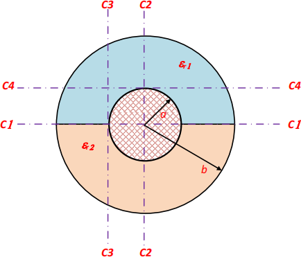 Figure 1
The problem conditions:
‐ Electrostatic problem
‐ Choose planar solution,
‐ Length units in millimetres, and
‐ Depth 1000 mm.
‐ Choose your mesh for not higher than 0.5 mm for improving the accuracy of the solution.
In your report,
Add vertical and horizontal contours (C1, C2, C3, and C4) to your schematic, then
a‐] Attach your schematic diagram with the required contours where the cable has one insulating material (Polypropylene insulator) with relative permittivity εr1 . (i.e. Both region 1 and region 2 have the same material Polypropylene insulator)
Plot the voltage distribution across contours C1 and C3. Plot the electric field distribution across contours. Comment on your results. Note: use a separate graph for each contour. [8 marks]
b‐] Find the cable capacitance using FEMM4.2 software for the cable given in part ‘a’, then confirm your answer analytically [7 marks]
c‐] Repeat part [a] by adding the second insulating material (PVC insulator)
with relative permittivity εr2. Plot the voltage distribution across contours C1, C2, C3 and C4. Plot the electric field distribution across contours. Comment on your results.
Note: use a separate graph for each contour [12 marks]
c‐] Plot the electric field tensor for part ‘c’ [3 marks]
d‐] Find the cable capacitance using FEMM4.2 software, then confirm your answer analytically [10 marks]
Note:
Five marks are allocated for report organisation/presentation.
Question 2 [50 marks]
A variable inductance can be represented by the magnetic circuit shown in figure (2). X represents the dimension in mm where x = (15 + m /4) mm and k factor equals 2.5. Choose the iron material from the FEMM4.2 library as a Mild‐steel M‐50. The number of turns of the coil is (70+m) turns.
The problem conditions:
‐ Electromagnetic problem
‐ Choose planar solution,
‐ Length units in millimetres, and
‐ Depth 1000 mm.
‐ Choose your mesh for not higher than 0.5 mm for improving the accuracy of the solution.
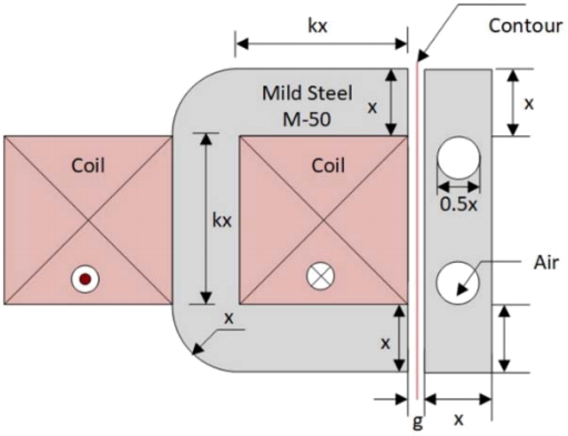 Figure 2
In your report,
1. Attach a schematic diagram with the required contours. Take the air‐gap ‘g’ = 1 mm.(Remember to add a boundary to your problem) [5 marks]
2. Calculate the coil current if the current density is (3.8+0.05m) A/mm2.
The filing factor is 55 %. [5 marks]
3. Calculate the coil inductance, (where  and
and  ), if the air gap
equals 1 mm and 5 mm (Note: ignore the air material in the plunger. This space is used to fix the plunger in the base; hence it is considered as air or non‐magnetic material) [5 marks]
4. Plot the flux distribution and flux tensor across the contour for the air gap limits (1 mm and 5 mm). [5 marks]
5. Plot the normal flux density component. [5 marks]
6. Measure the flux density in the air gap [5 marks]
7. Measure the inductance and compare it with the calculated one in number 2. Hint: integrate the vector A for the right coil (in and out current). You will get the result Henry*Ampere, and this result is per turn. Plot a relation between the inductance and the airgap in steps where g is the x‐axis and the inductance is the y‐axis (g starts from zero up to 5 mm, take 1 mm step) [15 marks]
Note:
Five marks are allocated for report organisation/presentation
2024-03-13