Hello, dear friend, you can consult us at any time if you have any questions, add WeChat: daixieit

Signal Processing and Spectral Analysis

Assignment 4

SDOF System

Consider a SDOF mass-damper-spring system:

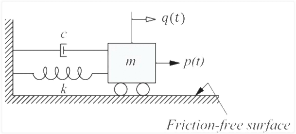
This system is governed by the following differential equation:

Subjected to the initial conditions:

Assume:

Problem 1: Obtain the closed form analytical solution of the Fourier Transform of load (right now an analog continuous-time function). Note that this is the causal LTI system and therefore  time value starts at 0 s. Plot:

a.   Load p(t) vs. t from t  ∈ [0,60] s.

b.   Absolute value of Fourier Transform of load |p(Ω)| vs. Ω from Ω ∈  [0,15]rad/s c.   Phase of Fourier Transform of input ∠p(Ω) vs. Ω from Ω ∈  [0,15]rad/s

Comment on the peaks that you observe in Fourier Transform magnitude plot. Where do these peaks occur and what do these peaks represent in your dynamic input load? You can use the following syntax for plotting:

Problem 2: Preferably using Mathematica, solve for the impulse response function by solving the differential equation for zero initial conditions subjected to unit impulse loading:

Subjected to the initial conditions:

Report the solution that you get by solving this differential equation and plot ℎ(t) vs. t from t  ∈ [0,60] s. Will this solution change if the external loading changed? Why?

Hint: Use “DSolve” command in Mathematica to solve for the differential equation. You’ll get HeavsideTheta[0] and HeavsideTheta[t] as part of your solution. Replace them with “HeavisideTheta[0]−> 0, HeavisideTheta[t]−> 1”. Your solution should match the closed form solution of ℎ(t) that we had obtained in class.

Problem 3: Using ℎ(t) obtained in problem 2, obtain the closed form analytical solution of the

Fourier Transform of impulse response (FRF). Note that this is the causal LTI system and therefore time value starts at 0 s. Plot:

a.   Absolute value of Fourier Transform ofFRF |H(Ω)| vs. Ω from Ω ∈  [0,15]rad/s b.   Phase of Fourier Transform ofFRF ∠H(Ω) vs. Ω from Ω ∈  [0,15]rad/s

Comment on the peaks that you observe in FRF magnitude plot. You’ll see that there is only 1 peak. Where does this peak occur and what does this peak represent in your impulse response? Why is there only 1 peak?

Problem 4: Preferably using Mathematica, solve for the response/output q(t) by solving the differential equation for zero initial conditions subjected to unit impulse loading:

Subjected to the initial conditions:

Report the solution that you get by solving this differential equation and plot q(t) vs. t from t  ∈ [0,60] s. Clearly mention the terms corresponding to the transient response and the steady state response.

Hint: Use “DSolve” command in Mathematica to solve for the differential equation. Notice that Mathematica may give you complex solution. However, we know that we have a real response function. We obtain that using the following command (after you have solved the differential equation):

Problem 5: Using q(t) obtained in problem 4, obtain the closed form analytical solution of the Fourier Transform of output/response, denoted by Q(Ω). Note that this is the causal LTI system   and therefore time value starts at 0 s. Plot:

a.   Absolute value of Fourier Transform of output |Q(Ω)| vs. Ω from Ω ∈  [0,15]rad/s b.   Phase of Fourier Transform of output ∠Q(Ω) vs. Ω from Ω ∈  [0,15]rad/s

Comment on the peaks that you observe in magnitude of the Fourier Transform plot. You’ll see that there are 3 peaks. Where does each of these peaks occur and what does each of these peaks  represent in your output? Why are there 3 peakspeak?

Problem 6: Obtain the cross-power spectral density (PSD) of input and output Syx (Ω), auto PSD of input Sxx (Ω) and output Syy (Ω). Plot each of their magnitude (absolute) plot and phase plot

for Ω ∈ [0,15]rad/second. Comment on peaks observed in each of these absolute plots and what these peaks represent.

Problem 7: Sample the input and output at frequency offs  = 100 Hz between t  ∈  [0,100] s and obtain discrete input p[n] and output q[n]. When we subject a system to input in the real world    (such as using shake table), the control system usually almost perfectly applies discrete input.

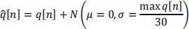
However, unlike input, acquiring output data is usually subjected to measurement noise. We simulate the noisy output sequence ̂(q)[n] that by adding zero-mean Gaussian noise:

Using the input sequence p[n] and the noisy output sequence ̂(q)[n], obtain:

1.   Plot discrete version of load p[n] and noisy output  ̂(q)[n] vs time vector for tn ∈

[0,100]s.

2.   Obtain DFT (using FFT algorithm) for the input sequence and output sequence. That is,

obtain, P[Ωk ] and Q(̂)[Ωk ] where Ωk   = N/2πfs   fork  = 0, … , N. Assume N equal to the

number of points in the sequence p[n] (or ̂(q)[n] since they are same length sequences).

Limiting your frequencies to Ωk   ∈  [0,15] Hz, plot the magnitude and phase of P[Ωk ] and

Q(̂)[Ωk ]. Here is a small snippet to help you:

3.   Obtain the estimated FRF sequence H[Ωk ]. Limiting your frequencies to Ωk   ∈  [0,15] Hz plot the absolute value |H[Ωk ]| and phase ∠H[Ωk ].

4.   Obtain the estimated cross power spectral density (PSD) sequencesyx [Ωk ]. Limiting your frequencies to Ωk   ∈ [0,15] Hz plot the absolute value |syx [Ωk ]| and phase ∠syx [Ωk ].

5.   Comment on the impact of measurement noise in estimating FRF and cross-PSD.