Hello, dear friend, you can consult us at any time if you have any questions, add WeChat: daixieit

MATH3027 Optimization 2021: Coursework 1

This is the first piece of assessed coursework for MATH3027 Optimization 2021. It is worth 20% of your final mark for the module.

The deadline for submission is Thursday 11 November at 10am. Your solution should be submitted electronically as a pdf file via the MATH3027 Moodle page. Late submissions will be subject to the usual penalties.

Since this work is assessed, your submission must be entirely your own work (see the University’s policy on Academic Misconduct). You can use, without acknowledgement, any of the material or code from the lecture notes or computer labs.

There are three questions below - you must answer all the questions. A handwritten and scanned solution is acceptable for question 1. For question 2 and 3 you must submit the code you use to find your solution. The easiest way to do this is to use Rmarkdown to create a pdf file.

This assignment will be marked out of 20.

Question 1 (4 marks)

Consider the function f : R² → R defined as

Find all of the stationary points of f, and classify them as local/global, strict/non-strict, and maxi-mum/minimum or saddle points.

Question 2 (10 marks)

Logistic regression is a form of statistical model used to model the probability of a binary event occuring as a function of some covariate information. In this question we will use logistic regression to predict the probability an individual has diabetes, using the covariate information

● pregnant: the number of times the individual has been pregnant

● glucose: the plasma glucose concentration in an oral glucose tolerance test

● pressure: Diastolic blood pressure (mm Hg)

We will use a subset of the Pima Indians dataset which were collected by the National Institute of Diabetes and Digestive and Kidney Diseases. You can download from Moodle and load it into R as follows:

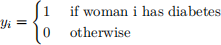
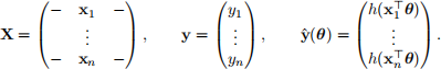
This contains information on n = 100 females of Pima Indian heritage, who are at least 21 years old. The vector y ∈ R¹⁰⁰ is our response vector, with yi the binary response for woman i,

The matrix X is a 100 × 3 matrix of covariate information:

Our aim is to build a logistic regression model to predict whether a patient has diabetes or not using the covariate information. The logistic regression model takes the form

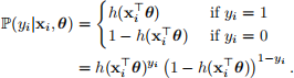
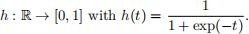
Here θ ∈ R³ is an unknown parameter vector that determines the importance of each piece of covariate information, and h is the inverse logit function:

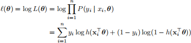
Our aim in this question is to learn the unknown parameters θ by maximum-likelihood estimation. The log-likelihood of the parameter θ is

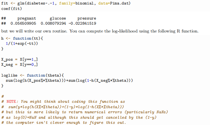
and we want to find the value of θ that maximizes (θ) (or minimizes the negative log-likelihood). There is an in-built command for doing this in R:

i. Show that the gradient of (θ) is

where

Write a function to compute the gradient. Your answer should be a vector of length 3. Check your answer numerically using a finite difference approximation. What is the gradient of (θ) at θ = (0, 0, 0)^T ?

ii. Implement the gradient descent method to find the maximum likelihood estimates of θ, using θ0 = (0, 0, 0)^T as an initial starting point. Use a fixed stepsize of = 10−6 , using

as the stopping criterion. How many iterations are required for the algorithm to converge? Plot the trajectory of the three parameters.

Note: we want to find the maximum here. The methods described in the notes were designed to find minima.

iii. What happens if you use a much larger step-size, e.g., = 10⁻⁵?

iv. Instead of using a constant stepsize, use the gradient method with backtracking with parameters s = 1, α = 0.25, β = 0.5. Does this work well? Try other values of s, α and β and discuss what you find.

v. Compute the Hessian matrix. Code a function to compute the Hessian and check your calculations numerically.

vi. Implement a Pure Newton’s method to find the maximum likelihood estimate of θ. Starting from θ0 = (0, 0, 0)^T, and using

as the stopping criterion, how many iterations does it take for the algorithm to converge?

vii. In statistics and machine learning, models are often regularized in order to improve the prediction accuracy by stopping overfitting. In Tikhonov or ridge regularization, instead of finding parameters to maximize the log likelihood (θ), we instead try to find parameter to minimize

Here λ is a parameter that controls the importance of the regularization term. If λ = 0 then this is equivalent to the maximum likelihood case. As λ → ∞, the parameter estimates tends to 0.

Implement a Newton method to solve the regularized logistic regression problem, and find the optimal θ when λ = 10³.

Plot the estimated value of the parameters as λ varies from 1 to 10⁶, using a log-scale for λ.

Question 3 (6 marks)

You wake up and find yourself on a strange planet. You find a spaceship and wish to fly home. But before you can safely do so, you need to estimate the acceleration due to gravity, g, and the drag coefficient of air-resistance, k. Thankfully, you remember your physics training and recall that for an object in freefall near the surface of the planet, the position of the object at time t, x(t) say, obeys the differential equation

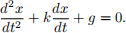
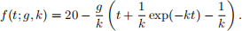
For parameters g and k, if we drop an object from a height of 20m at time t = 0 (so that x(0) = 20 and (0) = 0) then at time t, it will be at height

In order to estimate g and k, you set up an experiment, dropping a weight from a height of 20m, and then you observe (noisly) its location at times

Your measurements of the height of the weight at these times are

We want to use these measurements to estimate g and k. We will do this using non-linear least squares and solve the optimization problem

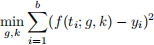
● Code a function to compute the objective function above as a function of θ = (g, k)^T. Compute its gradient and implement a function to calculate this. Check your answer numerically.

● Create a contour plot of

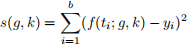
for g ∈ [1, 20] and k ∈ [0, 5].

● Implement a pure Gauss-Newton algorithm to find the optimal values of g and k, starting from g = 10, k = 2, and using as the stopping criterion. Report the number of iterations taken until convergence, the optimal values of g, k, and of the value of the objective at the optima.