MATH 120 — Project Activity 3
Hello, dear friend, you can consult us at any time if you have any questions, add WeChat: daixieit
MATH 120 — Project Activity 3
Hilly Dunedin
Dunedin is certainly not a flat city. In fact the extraordinary topography of this city must be taken into account for planning the city’s future, but also for understanding some of its present and past uses.
Part 1: Maximal Gradient of Baldwin Street
1.1: Introduction
During this activity, you will estimate the slope of Baldwin Baldwin Street at its steepest point using high-resolution elevation data obtained with the 3D laser scanning technology LiDAR (light detection and ranging). After extracting data from the LiDAR, you will reconstruct the height profile along Baldwin Street, quantify the gradient along the street and use numerical optimisation to estimate the maximum value of the gradient and the associated uncertainty. This will allow you to settle the debate once and for all on whether Baldwin Street is the steepest street in the world.
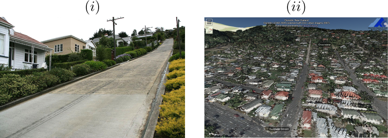
Figure 1: (i) Picture of the steepest part of Baldwin Street (source: CNN); (ii) Snapshot of Baldwin Street view point in Potree (source: Lidar 2009, School of Surveying Potree server).
1.2: Activity
Baldwin Street, located in North East Valley, Dunedin, has been recognised by the Guiness Book of Records as the steepest street in the world since 1987 with a gradient of 35% at its steepest point. As such, it has long attracted visitors to Dunedin, who usually climb the street as a pilgrimage walk. However, in 2019 Baldwin Street lost its record to Ffordd Pen Llech (Wales) with a gradient measured at 37.45%. After a review and appeal led by local surveyors, Baldwin Street reclaimed its title the following year. The surveyors argued that the gradient should be measured at the centre point of the street as opposed to the sides which makes a difference if the street curves, as was the case for the Welsh street. Along the street’s centre line, Baldwin’s Street’s gradient was remeasured to be 34.8% with modern technology in 2020, compared to 28.6% for Ffordd Pen Llech.
Light Detection And Ranging (LiDAR) is a geo-spatial surveying technique of 3D reality capture that de-termines the accurate position of points in 3D space by measuring the time-of-flight of a laser pulse emitted in a known direction. Airborne Laser Scanning (ALS) is a common application, whereby a LiDAR unit carried on-board an airplane scans the terrain underneath, collecting several million points per second to produce a dense and accurate picture of the topography called a point cloud. (You can find out more about the national liDAR capture program for New Zealand here.) The LiDAR dataset of Dunedin captured in 2009 is the main source for this exercise, with the product metadata available in the resources of this project providing key information about the capture, processing and quality of the data.
In order to visualise and interact easily with such large 3D point clouds, the School of Surveying maintains a Potree server. Potree is a user-friendly web-based interface that takes advantage of the 3D Graphical Library of web browsers (WebGL) to stream, navigate and measure massive point-cloud data efficiently in a geospatial environment. The 2009 LiDAR dataset can be accessed from the following url:
https://www.otago.ac.nz/surveying/potree/projects/MATH120_potree.html.
Several display and measuring tools are available in Potree, in particular a profiling tool that allows the 3D coordinates of data point along a custom path to be exported for analysis. Also note the navigation instruction upon the loading of the webpage.
Using the LiDAR data described here and available on the Potree server, answer the following question:
• What is the maximum gradient along Baldwin Street?
Although regression is a very useful technique to fit simple curves (e.g. lines) to data (see module 2), the real world can be messy and some datasets do not follow curves with known formulas. In such cases, curve fitting can still be achieved by using the techniques of smoothing and interpolation, which consists of fitting a smooth curve through the data with the goal of limiting rapid changes in its gradient. In this activity, you will need to create a smooth profile of Baldwin Street height along its centreline using a technique called smoothing spline. This can be done using computational software MATLAB with the built-in function fit. The interpolation function generated will allow you to estimate the height at regular points along the street, not just at the points where you have data. Once you have created the height profile, you will need to compute the gradient and find its maximum value. A MATLAB file is provided in Blackboard to guide you through the whole procedure.
In working through this activity, you will need to consider the following aspects:
• How can I export the data from Potree to be read into the MATLAB script file provided.
• What MATLAB tools (i.e. built-in functions) do I need and do I understand what they are doing?
• What assumptions do I make when using smoothing and interpolation tools?
• How can I quantify the uncertainty associated with my maximum gradient estimate?
• Is my estimate consistent with official measurements? If not, can I explain the discrepancy?
1.3: Hints & Tips
(a) We recommend you use a computer (desktop or laptop) with a mouse when playing around with the Potree server. It will make the navigation through the geospatial environment much easier.
(b) Interpolation works better when the data is relatively smooth. You can visualise profiles in Potree and try change the “width” value to try and include as many points as possible in your profiles while balancing smoothness issues.
(c) When exporting the LiDAR data, make sure the format is compatible with the software you use to process them, e.g. MATLAB. Note that you can read .csv files in MATLAB and convert them in MATLAB .mat data file. Select only the variables you need for subsequent computation.
(d) The point cloud data generated via the Potree server are not neatly ordered along the profile. The data need to be sorted in order to implement the smoothing spline method and compute the gradient. This step is already done in the MATLAB file provided using the command sort. DO NOT change this!
(e) There are several ways to perform smoothing and interpolation in MATLAB and there are a number of parameters/options that can be changed. Here we have implemented the smoothing spline technique using the built-in MATLAB function fit. The method fits a spline curve through the noisy data while minimising the noise. There is a smoothing parameter, describing how close from the data points the spline function is, that can be adjusted. It can take values between 0 and 1. Play around with it to see how it affects the performance of the fit.
(f) How do you calculate a gradient in % from an elevation profile? And how do you compute it in MATLAB? Have a look at the following built-in MATLAB functions: differentiate, gradient.
(g) Write down plenty of notes and save your data and figures as you work through the activity to help you for the final project report.
Part 2: Exploring a Section in Dunedin
2.1: Introduction
During this part of the project activity you will be investigating a section of Dunedin. You will be fitting the section to a plane and then finding different paths on this plane.
2.2: Activity
Sample an interesting section with no houses or trees in Dunedin using the “profile tool” of the potree soft-ware (https://www.otago.ac.nz/surveying/potree/projects/MATH120_potree.html). Set the width of the profile tool to a value suitable for your choice of section, for example, 50 m. Then export your data as a csv file.
You could choose a relatively flat section (for example from south Dunedin) or a relatively steep section (for example from North East Valley close to Baldwin Street or from the Otago Peninsula). Import the x-, y-, z-data from the csv file into MATLAB. This data describe the spatial 3d-position of every sampled point in your section. Notice that the y-axis of the software’s coordinate system is aligned with north, the x-axis with east, and the z-axis describes the altitude relative to sea level. The MATLAB code that is provided on blackboard should help you to import the data to MATLAB from the csv file (you might have to delete the very first row of your csv file to make this work) and should guide you through this lab activity. Use your exploration of this section, the plane fitted to it and the different paths on it to answer the following questions:
• What is the maximal gradient on the section?
• How does this exploration of the section help us understand the layout of Dunedin?
Possible topics of discussion, figures and data to be included are:
• the choice of the coordinate origin,
• the contour plot produced,
• the fit of your plane,
• the maximal, xy and zero gradient paths of the section.
2.3: Further instructions
1. You might have to redefine the origin of the coordinate system of your x-, y-, z-data in order to adapt it to your sampled section.
2. Make a contour plot of your data. You can use the contour or contourf commands (use help contour etc. to find out more). In order to use these commands you need to convert your data using the meshgrid and griddata commands as in indicated in the provided MATLAB * code. Discuss what you can learn from this plot.
3. Fit your data to a plane using the fit command (as also discussed in class). List your R2 -value and plane parameters and discuss what these tell you about the topography of your section.
4. Use the methods in lecture 32 to find the maximal gradient path, the x-y path of constant y and the xy-path of constant x and the zero gradient path of your fitted plane to your section from the plane parameters.
5. You need to write your values out to 2 sig. fig. so use the help section in MATLAB for the command fprintf to do this.
6. Write down plenty of notes and save your data and figures as you work through the activity to help you for the final project report.
2024-03-08