MATH 120 — Project Activity 2
Hello, dear friend, you can consult us at any time if you have any questions, add WeChat: daixieit
MATH 120 — Project Activity 2
Time series analysis and forecasting
Dunedin is not a stagnant city. Population, cost of living, average annual temperature are examples of quantities which are constantly changing over time. Understanding and quantifying the change a city has experienced in the past and being able to forecast future change are key to building a sustainable community.
Part 1: Empirical analysis
1.1: Introduction
You will perform regression analyses on two datasets to estimate (i) the rate of sea level rise in Dunedin, and (ii) the rate of rent increase in Dunedin over the last 25+ years. For each analysis, you will need to search and obtain relevant datasets, justify any pre-regression processing (e.g. smoothing or scaling), present the regression analysis using several empirical models, discuss/compare the results (including plots) and comment on the uncertainty.
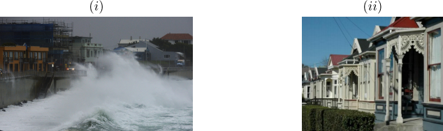
Figure 1: (i) Big waves hitting St-Clair sea wall in Dunedin (source: Otago Daily Times); (ii) Rental properties in Castle Street, Dunedin (source: Otago Daily Times).
1.2: Activity
Time series can be simply described as a list of data points ordered with time. This corresponds to the very natural way of collecting data that consists in recording how a quantity changes over time. Time series play a central role across all the sciences and any scientist should have a basic understanding of how to extract information through such datasets by conducting a regression analysis. Regression analysis seeks to estimate the relationship between the quantity measured and time (or more generally the independent variable). Simply speaking, regression attempts to fit a curve through data points when plotted against time.
Regression is typically composed of two steps: a qualitative one and quantitative one. The first qualitative step attempts to determine the type of relationship (e.g. linear, exponential, ...) relating the measured quantity to time. The second quantitative step numerically estimates the parameters of the relationship obtained in step 1. There is also a third (and often forgotten) step, which consists in quantifying how the first two steps performed. It is very important, however, as we need to know (i) if the type of curves chosen is appropriate for a given dataset, and (ii) the uncertainty of parameters estimated in step 2.
In this activity, you will perform two regression analyses with the goal of answering the following questions:
1. At what rate has sea level risen along Dunedin coast since the start of the 20th century and how is it projected to increase through the 21st century?
2. How has the cost of renting changed over the last 25 years in Dunedin?
These questions are open-ended and will require several steps to provide a nuanced and thorough answer. In working through each question, you will need to consider the following aspects:
• getting the data (what time series do I need? How do I obtain the time series? Where do I store the data?);
• plotting the data (what software do I need? What is the uncertainty on the data? Should I use linear or log scales?);
• pre-processing the data (is the data noisy? Are data points missing? Do I need to rescale the data?);
• choosing curve fitting models (what functions do I consider? Linear, polynomial, exponential, power, ...?);
• quantifying performance and uncertainty (how do I measure the goodness of fit? What is the uncer-tainty on the parameters?);
• deriving empirical models, i.e. equations that relates the quantity of interest to time.
1.3: Hints & Tips
(a) Make sure you understand and trust the source of all datasets you use. You should comment on the source of the data in your report and discuss any relevant information.
(b) Spend some time making simple quality control checks on your data, e.g. are data points missing, does the plot makes sense, etc?
(c) Start simple and incrementally refine your regression analysis. Think about what the simplest possible curve you can fit through the data is. Then upgrade your model and think about whether more information is gained in the process.
(d) Always check the units and magnitude of your estimates.
(e) Write down plenty of notes as you work through the activity to help you for the final project report.
Part 2: Forecasting Dunedin population
2.1: Introduction
In this activity, you will apply time-continuous models to predict the population of Dunedin in 2050 and 2100. This will require you to work with differential equations, use data to estimate the model parameters, implement numerical methods to solve the equations, discuss the results (validity, uncertainty, etc), and refine the models as appropriate.
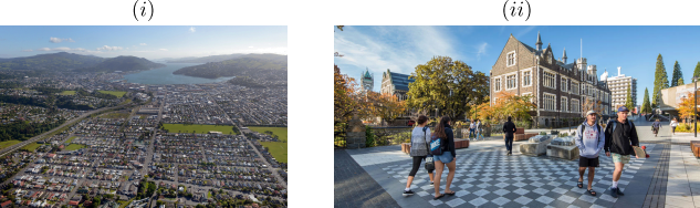
Figure 2: (i) Aerial view of Dunedin (source: Otago Daily Times); (ii) Students on campus (source: University of Otago).
2.2: Activity
Calculus (although often feared by students!) is one of the most powerful mathematical tools ever invented. It is arguably the most natural and simplest language that allows us to describe efficiently how the natural world behaves. Therefore, the orbit of planets around the sun and the concentration of a medicine in the bloodstream are equally well described by the language of calculus and its tools. At its core, calculus seeks to characterise how quantities that depend continuously on time change over time, especially when the change is not linear. The continuous change experienced by a quantity over time, or rate of change, is called the derivative.
Many models in science are constructed by relating the derivative of a quantity to the quantity itself. Such relationships are called differential equations. Although solving differential equations exactly can be diffi-cult, there are many numerical techniques available to approximate solutions using software, e.g. MATLAB.
In this activity, you will use the tools of calculus and associated numerical techniques to answer the following question:
What will the population of Dunedin be in 2050 and 2100?
As you work through this question, you should consider the following aspects:
• what are the quantities of interest and how can I model their change with time using a differential equation? What assumptions are made?
• What data do I need to inform the models (e.g. estimate the parameters) and where to find them?
• How do I convert the data into a format readable by MATLAB?
• How do I solve the differential equations (using ode45 or Euler) and what results do I plot?
• What is the uncertainty associated with my estimates?
• Can I validate my results against other data?
• How could the models be improved?
Although not a strict requirement, it is highly recommended that you use MATLAB to perform the computations needed for this activity. We have provided a script
2.3: Hints & tips
(a) Once you found data to inform your model, find a way to save them in a MATLAB .mat data file.
(b) Use the MATLAB code provided (DUD_pop_model.m) as a starting point for your MATLAB script.
(c) Consider a simple model first, e.g. exponential population growth with a single parameter, to get a feel about population trends. You can then improve the model with a more sophisticated population growth model, e.g. logistic growth with 2 parameters.
(d) Check out L21.1 and the associated MATLAB code to see how to implement the logistic growth model using ode45.
(e) One simple technique that can be used to estimate parameters is trial and error. Plot your model outputs against historical data for many different values of the parameters and decide visually which choice of parameters gives the best fit.
(f) If the model does not neatly fit the data, you can consider a range of values for the parameters and use it to estimate uncertainty on your final answer.
(g) Write down plenty of notes as you work through the activity to help you for the final project report.
2024-03-04
Time series analysis and forecasting