This homework is a hands-on introduction to parallel programming in distributed memory via MPI.

Your homework should be completed individually (not in groups).

Code and some parts of the handout are from UC Berkeley CS267 .

All instructions in this handout assume that we are running on PACE ICE. Instructions for logging in are in HW1.

Important: You CANNOT use OpenMP for this assignment. All of your parallel speedup must come from distributed memory parallelism (MPI).

Overview

In this assignment, we will be parallelizing a toy particle simulation (similar simulations  are used in mechanics, biology, and astronomy). In our simulation, particles interact by repelling one another.  A snapshot of our simulation is shown here:

The particles repel one another, but only when closer than a cutoff distance highlighted around one particle in grey.

Getting and running the code

Download from git

The starter code is available on Github and should workout of the box.  To get started, we recommend you log in to PACE ICE and download the code:

$ git clone https://github.com/cse6230-spring24/hw4.git

There are five files in the base repository. Their purposes are as follows:

CMakeLists.txt

The build system that manages compiling your code.

main.cpp

A driver program that runs your code.

common.h

A header file with shared declarations

job-mpi

A sample job script to run the MPI executable

mpi.cpp - - - You may modify this file.

A skeleton file where you will implement your mpi simulation algorithm. It is your job to write an algorithm within the simulate_one_step and gather_for_save

functions.

Please do not modify any of the files besides mpi.cpp.

Build the code

First, we need to make sure that the CMake module is loaded.

$ module load cmake

You can put these commands in your ~/.bash_profile file to avoid typing them every time you log in.

Next, let's build the code. CMake prefers out of tree builds, so we start by creating a build directory.

In the hw4 directory:

$ mkdir build

$ cd build

Next, we have to configure our build. We can either build our code in Debug mode or Release mode. In debug mode, optimizations are disabled and debug symbols are embedded in the binary for easier debugging with GDB. In release mode, optimizations are enabled, and debug symbols are omitted. For example:

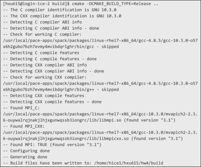
Once our build is configured, we may actually execute the build with make:

We now have a binary (mpi) and job script (job-mpi).

Running the code

You will need to test on at most four nodes for this assignment. To allocate two interactive nodes instead of just one (as we did in previous assignments), the syntax is simple:

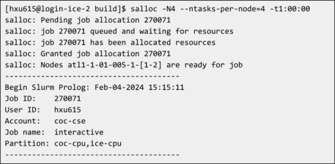
You now have a shell into one of the two allocated nodes. We recommend that you allocate only a single node and test on multiple MPI ranks with that node until you are ready to conduct a full scaling benchmark.

Unlike earlier assignments, you cannot directly run the executable from the command prompt! You must use srun or sbatch with the sample jobscript that we provide you. You can modify the jobscript to benchmark different runtime configurations. If you choose to run the binary using srun within an interactive session, you should set any environment variables in your interactive session to match the environment variables set by the jobscript. After you have done so, here's an example of how to run the simulation for two nodes:

(At first, the simulation time will be nothing because there is nothing implemented in mpi.cpp yet.)

To test on only a single node with 4 total MPI ranks, you can run:

Eventually, we want to scale up to 24 tasks per node, but before you try writing any parallel code, you should make sure that you have a correct serial implementation. To benchmark the program in a serial configuration, run on a single node with

--ntasks-per-node=1. You should measure the strong and weak scaling of your implementation by varying the total number of MPI ranks.

Rendering output and checking correctness

Refer to the HW2 handout.

Workflow tips

When you first start implementing the serial version, you only need to allocate one node and one task per node in your interactive jobs.

When testing your parallel version, first test with a smaller number of tasks per node still on one node (e.g., 2, 4, 8, etc.) using interactive nodes.

After debugging on small task counts interactively, you can submit job scripts for 4 nodes with 24 tasks per node.

Assignment

Implement the particle simulation in mpi.cpp by filling in the init_simulation, simulate_one_step, and gather_for_save functions.

The code walkthrough and description can be found in the HW2 handout.

It may help to check the MPI documentation.

Grading and deliverables

This homework has two deliverables: the code and the writeup.

Code

We will grade your code by measuring the performance and scaling of your MPI implementation.

Writeup

Please also submit a writeup that contains:

■   A plot in log-log scale that shows your parallel code’s performance and a description of the data structures that you used to achieve it.

■   A description of the communication you used in the distributed memory implementation.

■   A description of the design choices that you tried and how they affect the performance.

■   Speedup plots that show how closely your MPI code approaches the idealized p-times speedup and a discussion on whether it is possible to do better. Both   strong and weak scaling.

■   Where does the time go? Consider breaking down the runtime into computation time, synchronization time and/or communication time. How do they scale with p?

The exact problem sizes and process counts you should run on are given in the following sections. Please report on the process counts and problem sizes shown below in your writeup plots for uniformity between students. You are welcome to  try other sizes and process counts independently.

Here is an article with more details about strong and weak scaling.

Generating a parallel runtime plot

Please use the following sizes to generate a plot that showshow your parallel algorithm scales with problem size.

Scale the input size with four nodes and 24 tasks per node:

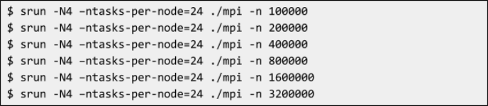
You should end up with a plot where the x axis is problem size (number of particles) and the y axis is runtime.

Generating a strong scaling plot

The simplest way to generate a strong scaling plot is to use different settings with srun:

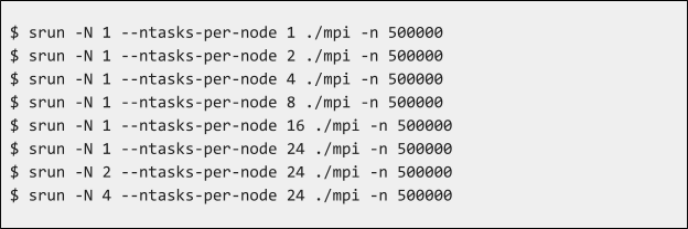
Each one of the numbers that will be output with commands like the above is one point in your speedup plot (for that corresponding number of processes). That is, the x axis is the number of processes, and the y axis is (multiplicative) speedup over the serial runtime. For a given point with x = p threads, the corresponding y point is T1/Tp (serial runtime over runtime on p threads).

Generating a weak scaling plot

Generating a weak scaling plot is the same as a strong scaling one except that you keep growing the input size proportionally with the resources.

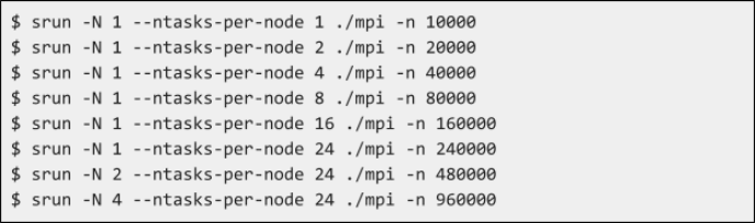
Each one of the numbers that will be output with commands like the above is one point in your weak scaling plot (for that size and number of threads).  That is, the x axis is the number of threads, and the y axis is (multiplicative) scaled speedup over the serial version. For weak scaling, scaled speedup is defined as efficiency * p, where p  is the number of threads, and efficiency is defined as T1/Tp.

Point distribution

Correctness of your implementation is a precondition to get any marks.

Raw performance - 1 points - includes:

- Normalized runtime compared to reference implementation.

Scaling - 3 points - includes:

- Scaling compared to reference implementation.

Writeup - 1 point - includes

- Plot of the parallel runtime on four nodes and 24 tasks per node, as described above.

- Description in the writeup of how you achieved the parallelization and how you implemented the communication.

- Strong scaling plot, as described above

- Weak scaling plot, as described above

That’s the end of this homework! Submit your writeup and code as described in the “Homework submission instructions” below: