BME 514 LAB 2 Spring 2024 PARAMETRIC & NON-PARAMETRIC SPECTRAL ANALYSIS OF EEG
Hello, dear friend, you can consult us at any time if you have any questions, add WeChat: daixieit
BME 514
LAB 2
Spring 2024
PARAMETRIC & NON-PARAMETRIC SPECTRAL ANALYSIS OF EEG
The basic purpose of this lab is to familiarize you with the 2 main approaches for spectral estimation of physiological signals: (1) Nonparametric – ie. FFT-based; and (2) Parametric – ie. model-based. A second purpose is to give you first-hand experience in dealing with non-stationarity in physiological signal analysis. In this assignment, you are given an EEG signal of duration 60 seconds, sampled at 100 Hz (Matlab file: eeg.mat). This signal was measured from the C3-A2 pair of leads in a sleeping patient with obstructive sleep apnea. The signal values are in units of microvolts.
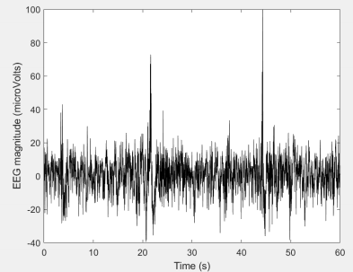
Your task is to analyze how the spectral content of this signal changes as a function of
time, since visual inspection (eg. big changes around 4s, 22s and 44 s) suggests that it is likely nonstationary. A simple approach is to divide up the signal into 12 nonoverlapping segments of 5 seconds, and to compute the spectra of successive segments using methods (1) and (2) described below, with the assumption of stationarity within each segment. In both cases, display the spectra as a function of time (it is best to use the same scale on the y-axis, so that differences in magnitude can be easily discerned).
Since both methods of spectral estimation are applied to the same data, there should be some degree of similarity across the corresponding results! Finally, based on the results from both approaches, briefly provide your interpretation of the behavior of the EEG signal.
(1) Nonparametric FFT-based approach:
The Blackman-Tukey method consists of first computing the biased autocovariance
function and then taking the DFT (FFT) of the autocovariance to obtain the power spectrum (Wiener-Khinchine Relation). Choose a suitable lag window (eg. Hanning) to reduce the effects of leakage - be sure to specify in your report which window you are using. Then, multiply the autocovariance function with the lag window (caution: the highest value, ie. 1, of the lag window, should be aligned with the highest value of the autocovariance function in order to preserve total power for the resulting spectrum!), and take the DFT of the result. Display the power spectra of the 12 segments – using the same ordinate (y-axis) scale so that comparisons can be made across spectra. Compute the power of the alpha (8- 12 Hz) and delta (1-4 Hz) bands for each of the successive segments, and display the time-courses of these derived variables.
(2) Parametric approach – Autoregressive (AR) modeling:
In this section, use the "lpc" function (https://www.mathworks.com/help/signal/ref/lpc.html) provided by the Matlab Signal Processing toolbox to determine the best AR model for each of the 12 segments. Begin by assuming an AR model of order 1. Compute the best-fit AR coefficients and the corresponding value of the Akaike Information Criterion (AIC).
Subsequently, increase the model order by 1, and repeat the computations until you arrive at the model order that minimizes AIC. Use the following definition of AIC:
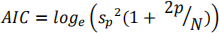
where p is the model order, sp2 is the residual variance and N is the total number of data points in the segment.
Based on the coefficients and the residual variance of the "best" model, compute the AR PSD function. Compute the power of the alpha (8- 12 Hz) and delta (1-4 Hz) bands for the successive segments, and display the time-courses of these derived variables.
IMPORTANT NOTE: In your report, make sure you explain briefly the steps you have taken to arrive at your final results. In both parts of the assignment, display your power spectra as functions of absolute frequency (in units of Hz). Since the power spectrum is symmetric about zero frequency, you need only display PSD values for frequencies > 0.
LAB REPORTS ARE DUE ON: WEDNESDAY FEBRUARY 14 AT 11:59 pm
2024-03-02