STAT3621 (2023-2024 Semester 2) Assignment 2
Hello, dear friend, you can consult us at any time if you have any questions, add WeChat: daixieit
STAT3621 (2023-2024 Semester 2)
Assignment 2
Please attach R code and the output together with your answers, and make sure your results are reproducible. Please combine the answers, R code and output into one file, preferably using R Markdown + knitr to produce a single HTML or PDF file.
1. Specifications are given for 387 new vehicles for the 2004 year. The variables recorded include price, measurements relating to the size of the vehicle, and fuel efficiency (cars.csv).
VARIABLE DESCRIPTIONS: Vehicle Name; Sports Car? (1=yes, 0=no); Sport Utility Vehicle? (1=yes, 0=no); Wagon? (1=yes, 0=no); Minivan? (1=yes, 0=no); Pickup? (1=yes, 0=no); All-Wheel Drive? (1=yes, 0=no); Rear-Wheel Drive? (1=yes, 0=no); Suggested Retail Price, what the manufacturer thinks the vehicle is worth, including adequate profit for the automaker and the dealer (U.S. Dollars); Dealer Cost (or "invoice price"), what the dealership pays the manufacturer (U.S. Dollars); Engine Size (liters); Number of Cylinders (=-1 if rotary engine); Horsepower; City Miles Per Gallon; Highway Miles Per Gallon; Weight (Pounds); Wheel Base (inches); Length (inches); Width (inches).
(a) Obtain a boxplot and histogram for suggested retail price and dealer cost respectively. Comment on your observations.
(b) Compare whether the median/distribution for suggested retail price and dealer cost differ or not. State the null and alternative hypothesis, test statistic, p-value and your conclusion clearly. Use α = 0.05.
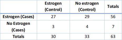
2. A study was carried out on post-menopausal women in City A. Cases of women with endometrial cancer were identified from this city. A control group was selected matched to the case on age and length of residence in city A. The medical question was whether endometrial cancer was related to estrogen use. Answer this question from the viewpoints of hypothesis testing (including to state the null and alternative hypotheses, the name of the test, the test statistic, and the p-value) and confidence interval (at significance level α = 0.05).
3. The file lbw.csv involves the low birth weight (lbw) data. This data set contains 189 observations on the following 10 columns:
low: a binary variable, which indicates whether the birth weight of a baby is under 2500g (low=1), or at a normal weight (low=0).
smoke: 1=history of mother smoking; 0=mother nonsmoker
age: age of mother: 14-45
race: categorical 1-3: 1=white; 2-=black; 3=other
lwt: mother weight (lbs) at last menstrual period: 80-250 lbs
ptl: number of false of premature labors: 0-3
ht: 1=history of hypertension for mother; 0 =no hypertension for mother
ui: 1=uterine irritability for mother; 0 no irritability for mother
ftv: number of physician visits in 1st trimester: 0-6
bwt: birth weight in grams: 709 - 4990 gr
(a) In these 189 individuals, how many mothers have history of smoking (smoke=1)? How many are nonsmokers (smoke=0)?
(b) Among the mothers with a history of smoking, how many of their babies indicate low birth weight (low=1)? Among the mothers who are nonsmokers, how many of their babies indicate low birth weight (low=1)?
(c) Denote the proportion of their babies with low weight (low=1) among mothers with history of smoking as !!. Denote the proportion of babies with low weight (low=1) among mothers who are nonsmokers as !" . Use a two-sample z-test to test the hypothesis:
H0: p1 = p2 v.s. H1: p2 ≠ p2.
(d) Find the 95% confidence intervals for p1 − p2.
4. The motor trend car road test data comprises fuel consumption and 10 aspects of automobile design and performance for 32 automobiles (1973–74 models). In R, please type data(mtcars) to load the data file. In “mtcars”, there are 32 observations on the following 11 (numeric) variables:
mpg Miles/(US) gallon
cyl Number of cylinders
disp Displacement (cu.in.)
hp Gross horsepower
drat Rear axle ratio
wt Weight (1000 lbs)
qsec 1/4 mile time
vs Engine (0 = V-shaped, 1 = straight)
am Transmission (0 = automatic, 1 = manual)
gear Number of forward gears
carb Number of carburetors
(a) Draw a scatter plot for mpg and wt. Report the Pearson correlation between mpg and wt?
(b) Check the normality of mpg by drawing the QQ plot. Then check the normality of mpg by performing Shapiro-Wilk’s test. Report the computed test statistic, p-value and your conclusion.
(c) Test whether the means of mpg are equal between the two Engine groups (i.e., vs =0 and =1). Report the computed test statistic, p-value and conclusion.
(d) Conduct the hypothesis test in (c) under the framework of one-way ANOVA model. Rewrite the hypothesis H0 and H1 in terms of ANOVA model parameters. Report the computed test-statistics, p-value and conclusion.
2024-03-01