Hello, dear friend, you can consult us at any time if you have any questions, add WeChat: daixieit

Practical 4 Development of a simple stratigraphic forward model

Note that this practical is assessed and work 50% of the module mark

The aims of this practical session are to:

•    Introduce you to the theory and practical considerations involved in constructing a simple stratigraphic forward model

•    Begin to apply the coding skills developed in the module sessions completed so far

•    Introduce you to some more basic elements of numerical forward models, including simple finite difference methods, numerical stability and grid boundary issues

•    Develop and assess your ability to use previously developed code fragments in functions to help construct a coding solution to a particular problem

•    Develop and assess your ability to develop code from an algorithm specified in a flowchart and following other guidance, as specified below

Instructions

1.    First, briefly recap the various content of the lecture and seminar session this week that introduced some of the theory of stratigraphic forward models, and went through an example of various aspects of one of these models.

2.    Pay particular attention to the flowchart and other instructions from the seminar presentation:

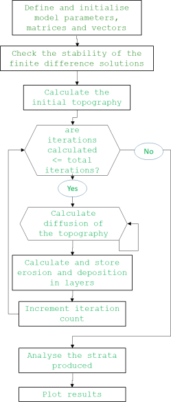
Your main task in this practical is to write code that implements this flowchart.

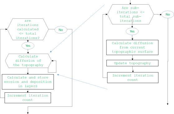
And remember, for the best possible solution, there should also a sub loop within the man time loop that calculates the diffusional erosion and depositional change to the elevation of a surface, using a shorter time step than used in the main loop that stores the layers of strata, so something like

Key elements in the model code should be:

•    Definition of an initial topography – see the initial topography shown in the seminar presentation, this is the one you need to use

•   Calculation of diffusional erosion and deposition across the topography through multiple forward-in-time steps

•    Representation of the strata produced by this erosion and deposition

•   A calculation of total eroded and total deposited volume per time step, with a warning  printed if these two values are not the same – differences could be due to an open grid boundary …

Details of all these elements were given and talked through in the seminar slides, and all of the initial variable values you need are actually defined for you in the

diffusionStratModeNotComplete.m code

3.    Following this guidance and the various other information provided in seminar material, and

using all the material from previous practical sessions, you should code the model, debug, test and run it to produce 100 layers, ideally with a shorter sub-loop iteration to ensure

numerical stability of the diffusion finite difference solution but note, this is additional work – you can still get a first-class mark without doing this.

4.    When the code is complete and working, you need to do some work to explore how the   model behaves and how it produces different results with different input parameters, so:

•    Assess how the strata changes with different values of the diffusion coefficient K, in m2  per time step because your grid size is in meters. Start with a value K= 5000m2 per time step as was set in the downloaded code, but also run examples with 2500, 50000, and 1000000 m2  per time step. Look carefully at the results in each case – how do the results change, is that what you expected and what does it tellus about how strata form with different rates of sediment erosion and transport? Most specifically, Is mass conserved on the grid for all these diffusion coefficient values? If not, what does this mean for the validity of the model? Could you still use it to make meaningful predictions of erosion and deposition?

•    Now write a very short report, maximum word limit 200 words for ENVS397, 500 words for ENVS597, to explain:

i.    how the modelled strata change with changing values of K,

ii.    Is mass always conserved in the model, and does it matter if it is or is not?

You should look at the marking rubric for this work before you complete this report, to make sure you understand how your report is going to be assessed and marked.

5.    Finally, AND VERY IMPORTANTLY you need save the Matlab code you have written as a Live Script .mlx file. If the code is not submitted correctly in this format it might not be marked,  and in that case you might get zero on this assessment. To submit correctly as a Live Script   .mlx file, do the following:

•     In the Matlab window where you have the .m file source code click on the save icon, thenon “save as” and select the Matlab Live Code files (*.mlx) option from the save   as type bar.

•    You should then find that your code reappears in a tab as a .mlx file. If you click on run and wait a while you will see output from the model appear on the right-hand  side of the screen, including the graphics plots

•    Now click on the text icon in the Live Editor menu bar and you can paste in your report text above the source code.

•    Also note that if you want to paste in images from the PowerPoint slides that

provide example output, perhaps because your code does not create all the

necessary graphics output, you can do this using the insert tab and then click on the image icon to upload saved images; you can save each image from the PowerPoint   file by right clicking on the image in the PowerPoint slide and selecting the “save as  image” option from the menu.  If you do this, please only paste at most one image    into the .mlx file, for example the cross section from the model run with the highest value of the kappa diffusion coefficient.

•    Make sure this is all saved, and you can then submit your .mlx Live Script file via the practical 4 assignment submission on Canvas.