闪电代写 -代写CS作业_CS代写_Finance代写_Economic代写_Statistics代写_代码代做_IT代写_加急帮助

Hello, dear friend, you can consult us at any time if you have any questions, add WeChat: daixieit

MATH2750 Introduction to Markov Processes Assessment 2

2023–2024

This computational worksheet is an opportunity to learn more about Markov chains using R. This practical doubles as Assessment 2, and is an assessed part of the course . This assessment counts for 3% of your final module grade.

You should write a report on your work (see Question 0 below), answering all the questions with explanations and figures where necessary, and showing any R code you used. Good formats for your report include PDF, Word document, or HTML. You work must be a report: do not just submit a list of R commands.

The deadline for submission is Thursday 14 March at 2pm. Late submissions up to Thursday 21 March at 2pm will still be marked, but the total mark will be reduced by 10% for each day or part-day it is late.

Your report will by marked out of 8, with 2 marks available for each of Questions 1–4 .

Question 0: Answer the questions on this problem sheet. Write up a short report on your findings, with answers to the questions. Make sure to include relevant graphs produced and the R code you used.

Remember that this is assessed work, and your report must be submitted by Thursday 14 March. You might like to look at the example report for Computational Worksheet 1 to see what a good report looks like. [HTML format][Rmd format]

We start by reading three functions into R by entering the entire text of the following code chunk. If you are using the Rmd version of this question sheet in RStudio, you can simply press the green “play” button next to the following code chunk. If you are reading the HTML version, you should carefully copy and paste the following code chunk into R.

# Produces a transition matrix for a Markov chain based on a parameter eps

TransMat <- function (eps) {

matrix (c (0.1 , 0.9 , 0 , 0 , 0 , 0 ,

0.4 , 0.2 , 0.4 , 0 , 0 , 0 ,

0 , 0.5 , 0 , 0.5 , 0 , 0 ,

0 , 0 , 0.5 , 0.5-eps, eps, 0 ,

0 , 0 , 0, eps, 0.3-eps, 0.7 ,

0 , 0 , 0 , 0 , 0.5 , 0.5),

nrow = 6 , ncol = 6 , byrow = TRUE)

}

# Simulates a Markov chain with transition matrix P for N steps from X0

MarkovChain <- function(N, X0, P) {

X <- rep (0, N) # empty vector of length N

space <- nrow (P) # number of points in sample space

now <- X0

for (n in 1:N) {

now <- sample (space, 1 , prob = P[now, ])

X[n] <- now

}

# Finds the stationary distribution of a Markov chain

StatDist <- function(P) {

LeftEigen <- eigen (t(P))

statmeas <- LeftEigen$vectors[, 1] # Unnormalised stationary measure

statmeas / sum (statmeas) # Normalised stationary distribution

}

It is not important that you understand how these functions work, but you do need to know what they do.

The first function TransMat() produces a transition matrix

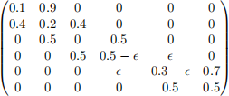
for some value of the parameter ϵ .

The second function, MarkovChain(), simulates a Markov chain. For example, MarkovChain(10, 2, P) simulates a Markov chain with transition matrix P, starting from state 2 for 10 steps.

The third function, StatDist(), calculates a stationary distribution for a given transition matrix. This function works for any irreducible Markov chain on a finite state space – it may behave strangely for nonirreducible Markov chains.

We will be investigating the Markov chain with ϵ = 0.1.

Question 1. Using the function TransMat(), produce the transition matrix for ϵ = 0.1. Using the function MarkovChain(), simulate N = 100 steps of this Markov chain starting from X0 = 1 . Check it has worked, perhaps by plotting a graph or examining the vector produced. Comment on what you find.

You will presumably want to try something like this:

eps <- 0.1

P <- TransMat (eps)

N <- 100

X0 <- 1

X <- MarkovChain(N, X0, P)

plot(X)

If you plot a graph of the Markov chain, you may want to add extra options to label axes, add lines to the points, include the point X0 = 1 etc, as in the previous practical. See the help file ?plot to remind yourself.

Question 2. Calculate the proportion of time spent in each state. What if you choose N to be very large? How does this compare with the stationary distribution? Relate what you have found to a result in the course.

One way to count the number of visits to each state is to use the table() function, although you may be able to think of a different way. The command table(X) gives the number of entries in a vector X that have each value. (If your Markov chain did not visit every state, table(factor(X, 1:6)) will ensure it counts 0 for the unvisited states.)

num_visits <- table (factor(X, 1:6))

proportion_time <- # your code here

Remember that you want the proportion of time spent in each state, not just the number of visits.

It may also be helpful to illustrate your example with a graph. You will want to give your plot a title, label the axes, and so on.

You can compare this with the stationary distribution produced by StatDist().

stationary <- StatDist(P)

rbind (proportion_time, stationary)

You might find it useful to draw a bar chart comparing the proportion of time spent in each state with stationary distribution. The basic code to draw a bargraph works like this:

barplot (rbind (proportion_time, stationary), beside = TRUE , legend.text = TRUE)

You might want to label your plot or change the legend text – reading the help file ?barplot may be helpful here.

Make sure you have checked what happens with your code for a large value of N – something like N = 100 000 or even more might be appropriate.

Remember that if you use a certain routine many times, it can be helpful to write it into a function.

Question 3. For each state, estimate the expected return time µi . What do you expect the answer to be? How does your result compare with this?

A useful function here might be the which() function, where which(v == x) gives a list of all the coordinates i at which a vector v took on a particular value vi = x. So, for example, which(X == 3) will give a list of all the times when the Markov chain was in state 3.

Another useful function is the function diff(), which produces the consecutive differences of a vector; so, for example,

diff(a,b,c,d, e) = (b − a, c − b, d − c, e − d).

Can you use which() and diff() together to find all the return times to your chosen state, and thus calculate the mean return time?

Again, a chart might be a useful way of making a comparison.

Question 4. What do you think would happen if you were to repeat the above exercises with ϵ = 0.01? What about ϵ = 10 −6 ? What about ϵ = 0? Explain your answers.