Hello, dear friend, you can consult us at any time if you have any questions, add WeChat: daixieit

MN-3505 Asset Management

Portfolio Theory – Practice Set

Question

You have been provided with the following information about the stocks of two companies:

Required:

1. Calculate the Minimum Variance Portfolio (MVP). and return and standard deviation for this portfolio  

2. Solve the weights for the optimal risky portfolio (ORP) and optimal final portfolio (OFP)  

3. Estimate the return and standard deviation for the optimal risky portfolio (ORP) and optimal final portfolio (OFP).

4. Suppose you had £1,000,000, how much money would you invest in each of the three assets i.e. RF, JPM and AMZ? [Hint: 69% in ORP and 31% in RF; out of 69% in ORP split 72.73% (JPM) and 27.27% (AMZ)] 

Solution

Let’s just assume JPM is denoted as A and AMZ as B

Summary of Answers: 

(1) Minimum Variance Portfolio

Step – 1 Identify weights for both securities (i.e. how much to be invested in each)

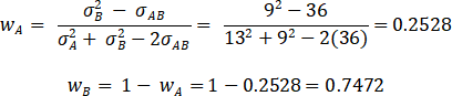
This means that a portfolio with 25.28% funds invested in A and 74.72% invested in B will have minimum possible variance.

Step – 2 Estimate Portfolio Returns for the Minimum Variance Portfolio

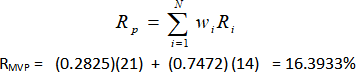
Step – 3 Estimate Portfolio Variance Standard Deviation for the Minimum Variance Portfolio

(2) ORP and OFP – weights

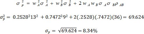
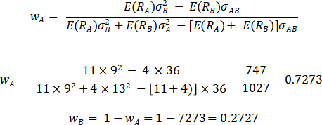
2(i) Optimal Risky Portfolio (ORP) – weights

Step – 1 Let’s estimate excess returns for both securities i.e. E(R_A) and E(R_B)

E(R_A) = R_A – R_F = 21 – 10 = 11%

E(R_B) = R_B – R_F = 14 – 10 = 4%

Now estimate the Return and Standard Deviation based on these weights. See 3(i) below

2(ii) Optimal Final Portfolio (OFP) – weights (combination of ORP and RF)

Please do not enter the values in percentage here as the coefficient of risk aversion (A) is scaled in line with the decimal values. If you enter percentage values of returns and SD, your answer will be incorrect. Best way to do this step is to take highlighted values i.e. R_ORP, R_f and SD in decimals.

 

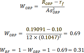
Now estimate the Return and Standard Deviation based on these weights. See 3(ii) below

(3) ORP and OFP – Portfolio Returns and Portfolio SD for ORP and OFP, respectively.

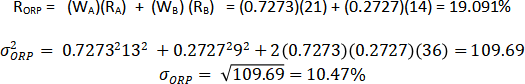
3(i) Optimal Risky Portfolio – Return and Standard Deviation (Weights here are calculated in 2(i) above. 

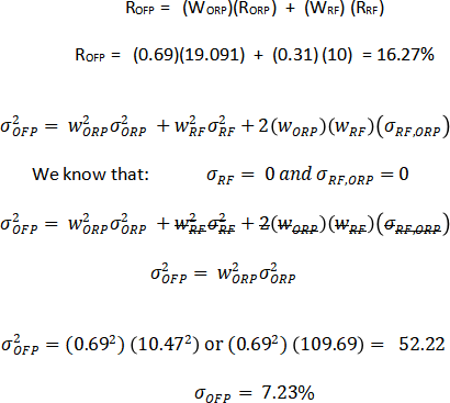
3(ii) Optimal Final Portfolio – Return and Standard Deviation (Weights here are calculated in 2(ii) above. 

(4) ORP and OFP – Portfolio Returns and Portfolio SD for ORP and OFP, respectively.