Hello, dear friend, you can consult us at any time if you have any questions, add WeChat: daixieit

PPHA311

ProblemSet5

Winter2024

1 The Oregon Health Insurance Experiment, Revisited (16 points)

In this problem, you will continue to work with the data from Problem Sets #1 and #3. Please refer back to Problem Set 1 for variable definitions.

For this assignment, you can refer to any output that comes from the lm() function. For question 9, you can also use the ivreg() function.

1. In Problem Set #2 Q2, we tested for heterogeneity across different groups by running separate regressions of visit dr on treated, controlling for numhh list, and examining whether or not we could reject whether the treatment effect for each group was statistically different from zero. We will revisit this by examining whether or not the treatment effects are statistically different from each other. Run the following four regressions.

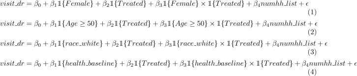
where 1{Female} is an indicator for identifying as female, 1{Age ≥ 50} is an indicator for being aged 50 or older, 1{race white} is an indicator for being White and non-Hispanic, and 1{health basline} is an indicator for having a diagnosis of a major health condition pre-lottery.

Interpret the β₃ coefficients you estimate (point estimates and statistical significance). How do your results compare with what you found in Problem Set #3, Q2? (3 points)

2. Consider the variable ever medicaid, which reports whether someone actually enrolled in Medicaid coverage since the lottery. Did everyone who won the lottery take up Medicaid? Calculate the mean of ever medicaid among those who won the lottery.

Are there some people who lost the lottery who take up Medicaid? Calculate the mean of ever medicaid for those that lost the lottery.

Now, recall the key regression from Problem Set #1:

Y = β₀ + β₁treated + ϵ

We have been interpreting the coefficient on treated as the causal effect of winning the Medicaid lottery. Is this likely to be the same as the causal effect of actually receiving Medicaid? (1 point)

3. Estimate the following “First-stage” regression:

ever medicaid = α₀ + α₁treated + α₂numhh list + e (5)

Interpret the regression coefficient on α₁. (1 point)

4. Is treated likely to be a valid instrument for ever medicaid in terms of the three key assumptions: instrument relevance, independence assumption and the exclusion restriction? If there is a specific statistical test that helps validate the plausibility of each assumption, please refer to this evidence (3 points)

5. One possible way to estimate the effect of receiving health insurance is the ratio of the coefficient on the instrument in the reduced form model to the coefficient on the instrument in the first-stage regression. Let’s again focus on the outcome count visit dr. Recall, the reduced form is the regression we’ve already been running in Problem Sets #1 and #3:

count visit dr = β₀ + β₁treated + β₂numhh list + ϵ (6)

Calculate and report the ratio of the reduced form to the first stage. Note that technically, we should use the same number of observations in our first-stage and reduced form, so you should calculate the first stage excluding rows with missing values of count visit dr. Interpret your result (2 points)

6. Let’s next estimate the IV model via two-stage least squares (2SLS). Manually estimate the two stages:

(a) First-stage: Run the regression  and compute predicted values: 

(b) Second-stage: Run the regression count visit dr = β₀+β₁ever\medicaid+β₂numhh list+ ϵ

Again, you should only estimate the first stage on the subset of the data where count visit dr is not missing. How does your result compare to the previous estimate? You can now also conduct inference–is the IV estimate statistically significant? (2 points)

7. Now, we will try including all the baseline characteristics as controls. However, unlike in Problem Set #3, let’s account for a non-linearity in age by including a quadratic term, age².

Thus, the full-set of controls become: numhh list,female,age,age²,race white,hs degree,college degree,health baseline.

Re-estimate the 2SLS model including these controls and compare the size of the coefficient on ever medicaid and the standard error to the results in part (6). (2 points)

8. Let’s calculate the IV estimates for all the endline outcomes now, including the full set of controls.

To make things easier, you are welcome to use the IV R command, ivreg. You will first need to install the R package AER. Do this by typing into R: install.packages(“AER”). Then load the package: library(“AER”).

For each of the endline outcomes, run the IV regressions including the controls. Fill in the table below with your results. Discuss your findings, including their precision. (2 points)