Hello, dear friend, you can consult us at any time if you have any questions, add WeChat: daixieit

Homework 5 - Fitting and Visualizing Regressions

IRE379

Figure 1: Bathe in the balmy weather data

1 Fitting and visualizing a regression model

1.1 Reading the data

The file weather_5cities.csv contains average daily temperatures from five different cities. Read it into memory. What timespan does the data cover?

1.2 Examine the histograms

We will use linear regression to model the temperature in Ottawa (Y) as a function of the temperature in Toronto (X). Before we begin, use ggplot() to examine the histograms of temperatures in Ottawa and Toronto to satisfy yourself that there are no unusual observations or anything else troubling about the data.

1.3 Examine the scatterplot

Before we fit a regression line, generate a scatterplot using the predictor variable (temperature in Toronto) on the x-axis and the outcome variable (temperature in Ottawa) on the y-axis.

1.4 Fit the regression model

We usually write regression functions like this: Yi = β0 +β1Xi +ui . Yi is the outcome, and Xi is the predictor. Fit this regression function to our data using lm_robust() from the estimatr package. (You will need to install the estimatr package if you have not already.) What does the estimated intercept (βˆ 0)? What is the estimated slope (βˆ 1)?

1.5 Compute predicted values of the outcome

Calculate the predicted value (written as Yˆ ) of the temperature in Ottawa when the temperature in Toronto is 0◦ . How about when the temperature in Toronto is 20◦ ? (Note: this only requires simple arithmetic.)

1.6 Add the regression line to the scatterplot

We can add a linear regression line to our scatterplots by adding this geom geom_smooth(method='lm', se=F) to our ggplot() call. Here, “lm” stands for linear model. Add this to your scatterplot from 1b. Do your predicted values from the previous step fall on the regression line? At what temperatures does the regression line look like a more accurate predictor of temperatures in Ottawa? At what temperatures is it a less accurate predictor?

1.7 Saving plots to files

Finally, save your plot to a PDF file. Use ggsave("ottawa_toronto.pdf", width=?, height=?) to save the latest call to ggplot() to a PDF. (width = 5 and height = 3 often looks nice, but feel free to play around.) No need to upload with your homework—this is just to practice saving your plots.

1.8 Customizing the visualization

Try these extensions to your ggplot():

• Add the points relating temperatures in Vancouver (Y) to temperatures in Toronto (X) to the same plot as our plot of Ottawa. You can do this by adding a geom_point() that maps the y aesthetic onto the column: vancouver.

• Change the color of the new Vancouver points to red

• Change the shape of the new Vancouver points to little triangles (see: http://www.sthda.com/english/wiki/ggplot2-point-shapes)

• Improve the contrast by removing the gray background (one option is to add theme_minimal()).

2 Vancouver, Fiji, and Melbourne

Let’s use visualization to guess at the regression parameters before fitting regressions. We will use some of the other cities in weather_5cities.csv.

2.1 How well do Toronto temperatures predict Vancouver temperatures?

Examine your scatterplot of Toronto (x) and Vancouver (y) temperatures from problem 1.8 (Make sure the Toronto–Vancouver points .. Based on the shape of the data, do you expect the slope (βˆ 1) relating Vancouver temperatures to Toronto to be greater or less than the estimated slope for Ottawa and Toronto from problem 1? Why? Fit the regression model using lm_robust() and examine the estimated slope to check your intuition.

2.2 How well do Toronto temperatures predict Fiji temperatures?

Start a new ggplot() that shows a scatterplot of Toronto (x) and Fiji (y) temperatures. (Do not add a regression line yet.) Roughly what do you expect the intercept (βˆ 0) of the regression fit to be? Why? Fit the regression model using lm_robust() to check your intuition.

Finally, add a regression line to your plot using geom_smooth(method='lm', se=F).

2.3 How well do Toronto temperatures predict Melbourne temperatures?

Make a scatterplot of Toronto (x) and Melbourne (y) temperatures. Do you expect the slope (βˆ 1) to be positive or negative? Why? Roughly what do you expect the intercept (βˆ 0) of the regression fit to be? Fit the regression model using lm_robust() to check your intuition.

Using you knowledge of weather/seasons, why does this regression line slope the way it does?

Finally, add a regression line to your scatterplot.

3 Extra credit. Calculate the regression coefficients by hand

Key Concept 4.2 in Stock and Watson provides an algebraic definition of the OLS regression slope βˆ 1 and intercept βˆ 0, where ¯X is the sample mean of X and Y¯ is the sample mean of Y. The slope of the regression line is given by:

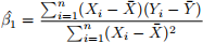
After computing βˆ 1, you can compute the intercept βˆ 0:

Try using this formula to compute the regression slope and intercept relating Toronto (X) to Melbourne (Y) by hand. Start by storing the Toronto temperatures in the vector x and the Melbourne temperatures in the vector y. For example, if your tibble was named cities, you should start with:

x = cities$toronto

y = cities$melbourne

Notes

The notes section contains additional information about the problem set. It does not require any action on your part.

Building the daily temperature data for this homework