Hello, dear friend, you can consult us at any time if you have any questions, add WeChat: daixieit

STAT512

Assignment 3

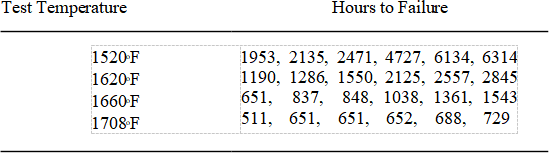
In the previous homework assignment, an experiment was described in which a temperature-accelerated life test was performed for a type of sheathed tubular heater.  Six heaters were tested at each of four temperatures: 1520^oF, 1620^oF, 1660^oF and 1708^oF.  The number of hours to failure was recorded for each of the 24 heaters in the study.

The primary learning outcome was to learn how to assess the model assumptions for a completely randomized design with a one-way treatment structure.  Recall that the assumptions were violated for the above data and a transformation was performed. For this question, we will return to the analysis of the means, first assessing the global test of equal means and subsequently assessing contrasts of the means.  When using SAS Proc GLM, we will analyze the transformed response (hours until failure), using the inverse square-root transformation.  

The treatment factor, Temperature, is a quantitative factor.  Although ANOVA models treat all factors as qualitative, it is possible, through contrasts, to assess whether there is a trend in the response means over the levels of the factor.  This can be seen through the scatterplot of the mean inverse square-root of hours of life (first graph) plotted against the factor levels and the scatterplot of the mean hours of life (second graph) plotted against the factor levels.

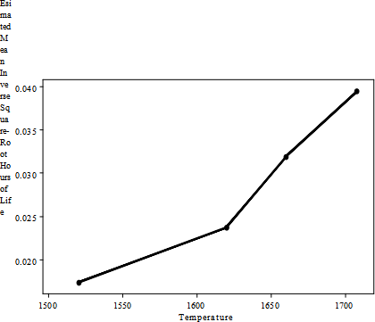
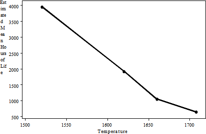
Both graphs show a trend, although in different directions.  For the most part the trend is linear (straight line). Other forms of a trend are also possible: quadratic, cubic, etc. Determining whether a trend is actually present and not an artifact of random sampling, requires orthogonal polynomial contrasts.

By the end of this laboratory, you will be able to determine the coefficients for orthogonal polynomial contrasts for any spacing of the quantitative factor levels.  You will also be able to assess whether there are trends in the mean response by computing the contrasts.

The SAS Proc GLM code for the life testing data is shown below.

data lifetest;

input Hours Temperature Replicate @@;

InvSqrt_Hours = 1/sqrt(Hours);

cards;

1953 1520 1 2135 1520 2 2471 1520 3 4727 1520 4 6134 1520 5 6314 1520 6

1190 1620 1 1286 1620 2 1550 1620 3 2125 1620 4 2557 1620 5 2845 1620 6

 651 1660 1  837 1660 2  848 1660 3 1038 1660 4 1361 1660 5 1543 1660 6

 511 1708 1  651 1708 2  651 1708 3  652 1708 4  688 1708 5  729 1708 6

proc glm data = lifetest;

class Temperature;

model InvSqrt_Hours = Temperature;

contrast "Linear Trend" Temperature -0.773254 -0.050587 0.2384801 0.5853604;

run;

Use SAS Proc GLM to compute the analysis of variance for these data, along with the linear trend and report the results on the next page.

Most texts on the design of experiments provides the orthogonal polynomial contrast coefficients for factors having between 2 and 5 levels, but only for equally spaced factor levels.  The following SAS Proc IML program will compute the orthogonal polynomial contrasts for any spacing of the factor levels.

OPTIONS LS=72 pageno = 1;

title "Construction of Orthogonal Polynomials Using SAS Proc IML";

title2 "Orthogonal Polynomials for Equal Spaced Levels";

title3 "Temperature Levels: 1520, 1620, 1660 and 1708";

/***

ENTER INTO VECTOR A THE FACTOR LEVELS FOR WHICH THE ORTHOGONAL POLYNOMIALS ARE REQUIRED. THE LINEAR ORTHOGONAL POLYNOMIAL IS ROW #1, QUADRATIC IS ROW #2, CUBIC IS ROW # 3, ETC. CONTRASTS ARE HORIZONTAL.

***/    

PROC iml;

= {1520 1620 1660 1708};

Nentries = ncol(A)- 1;

Labels = {Linear Quadratic Cubic Quartic Quintic Sestetic Septupic Octupic};

Labels = Labels[ ,1:Nentries]`;

B = ORPOL(A);

B = B[ ,2:(Nentries+1)]`;

PRINT "Input Vector of Factor Levels" A;

PRINT "";

PRINT "Orthogonal Polynomials";

PRINT  B [rowname = Labels];

RUN;

The coefficients for the linear trend that result from running this program (in part) are as follows:

LINEAR    -0.773254 -0.050587 0.2384801 0.5853604

Run the Proc GLM code with the linear orthogonal polynomial contrast and report the results below:

1) Test for a linear trend in the mean hours of life across temperature.

a) H_o: No linear trend present

b) H_a: Linear trend present

c) F =                                       Pvalue =

d) Reject H_o if F >                    or Pvalue <

e) Conclusion:

Run the program for producing the coefficients for the orthogonal polynomial contrast.  Substitute the quadratic and cubic contrast coefficients into the SAS Proc GLM code and run the analysis.  Report the results in parts 3 and 4 below.

2) Report the coefficients for the quadratic and cubic orthogonal polynomial contrasts.

                        Temperature

                        1520                   1620           1660                   1708

Quadratic

Cubic

3) Test for a quadratic trend in the mean hours of life across temperature.

a) H_o: No quadratic trend present

b) H_a: Quadratic trend present

c) F = Pvalue =

d) Reject H_o if F > or Pvalue <

e) Conclusion:

4) Test for a cubic trend in the mean hours of life across temperature.

a) H_o: No cubic trend present

b) H_a: Cubic trend present

c) F =              Pvalue =

d) Reject H_o if F > or Pvalue <

e) Conclusion: