Electronic Structure Theory Exercise 6
Hello, dear friend, you can consult us at any time if you have any questions, add WeChat: daixieit
Electronic Structure Theory
Exercise 6
Due: Friday Week 8, 12 pm
1 Aims
In this exercise, you will use density functional perturbation theory (DFPT), as im- plemented in the Quantum ESPRESSO package, to calculate phonon dispersions and density of states for bulk silicon. You will then compare your results to experimentally measured properties of silicon that are related to its lattice vibrations.
2 Instructions
2.1 Preparation
Copy and unpack the QE input file archive into an appropriate sub-directory of your user account.
user@login:˜> mkdir exercise −6
user@login:˜> cd exercise −6
user@login:˜> cp /home/dc158/dc158/shared/ input ![]() files . tar . gz
files . tar . gz
.
user@login:˜> tar −zxvf input files . tar . gz
user@login:˜> cd Exercise −6/inputs
Have a look at the job script QE-phonon. slurm. DFPT as implemented in QE is done as a sequence of calculation steps (see also week 6 lectures):
1. A SCF calculation to obtain ground state wave functions and eigenvalues on a regular k-point mesh (using si.scf. in).
2. A calculation of the DFPT matrix elements on a regular q-point grid; this grid need not be the same as the SCF k-point grid (si.ph. in).
3. A Fourier transform from q-space to real space, to obtain the interatomic force constant matrix from the dynamical matrix (q2r. in).
4. Postprocessing calculations to obtain arbitrary phonon dispersions (si. ph-disp. in) and density of states (si. ph-dos. in); the latter, again, on a regular q-point grid, but this can now be much denser. (The last two steps essentially represent a Fourier interpolation of discrete data residing in reciprocal space).
3 Tasks
3.1 Phonon convergence tests
Run the job script. The calculations will eventually produce two important outputs, si. ph-disp. gp and si. ph-dos.dat. These contain, respectively, the phonon disper- sions along the special path designated in si. ph-disp. in and the phonon density of states on the grid specified in si. ph-dos. in, in units of wave numbers (cm− 1 ). Plot both dispersion and DOS - you should find all-positive phonon frequencies, with three acoustic branches (ω → 0 around the Γ point) and three optical branches at higher frequencies. Does the DOS correspond to the dispersion data?
How does the DOS change if the q-point grid is changed (a) in si. ph-dos. in (i.e., the postprocessing), and (b) in si. ph. in (i.e., in the DFPT calculation)? Beware that the DFPT calculations are the bottleneck here, and large q-grids might take a longer time to finish. Once the DFPT calculation has run through, postprocessing can be done interactively on Cirrus1. What q-grid do you deem necessary for the DFPT calculation to obtain both converged phonon DOS and dispersions?
3.2 Phonon observables
From the phonon dispersions, we can now estimate both the longitudinal and the trans- verse sound velocity in silicon. Determine the slopes of the acoustic phonon branches as they emerge from the Γ point, and use those to calculate the two sound velocities via ω = ck. How do they compare to experimental data? How does the triply degenerate optical mode at Γ compare to the Raman scattering signal of crystalline silicon?
We can also compare the calculated phonon dispersion throughout the Brillouin zone to data measured in neutron scattering. Use the data by Kulda et al. (Physical Review B 50, 13347 (1994)) to assess the validity of your calculations, preferrably by plotting the neutron data together with your dispersion curves. To annoy us, the authors in that paper denote reciprocal space directions based on the conventional (cubic) reciprocal unit cell, and not on the primitive Brillouin zone. In Figure 1 I show how the two lattices and coordinate systems are related.
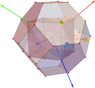
Figure 1: Brillouin zones of face-centered cubic lattice: for the primitive unit cell (outher polyhedron), and the conventional cell (inscribed cube). Reciprocal lattice vectors for primitive/conventional cells are indicated by solid/dashed arrows. Special points, expressed in conventional coordinates, are X : (1, 0, 0) (orange); K : (3/4, 0, 3/4) (blue); L : (1/2, 1/2, 1/2) (green).
4 Submission
Submit a summary of your results, addressing the questions posed in the previous section. Submit a single document (preferrably PDF) including figures and discussion.
5 Marking Scheme
. Si phonons: DOS and dispersion plots, convergence of q-grid in postprocessing and within DFPT, discussion. [24]
. Si observables: sound velocities, comparison to Raman and neutron data, discus- sion. [16]
Total marks: 40, count for 20% of the course grade.
2024-02-17