1  Aims

In this exercise, you will use the Quantum ESPRESSO (QE) density functional theory package to calculate more advanced ground-state properties of different materials.  These include electronic densities of states and band structures, estimates of pressure-induced phase transitions, and estimates of elastic constants.

You will perform these calculations on materials you have already encountered, silicon, quartz, and the α- and β-phases of tin.

2  Instructions

2.1  Preparations

Log into Cirrus.  Copy the QE input file archive into an appropriate sub-directory of your user account and unpack it.  Also remember to lookup your convergence test results from the previous exercise, for both silicon and the two tin allotropes.

user@login:~>  cp  /home/dc158/dc158/shared/input_files. tar. gz

.

user@login:~>  tar  -zxvf    input_files. tar. gz

user@login:~>       cd  Exercise -5/inputs

Have a look at the QE input files and job scripts.  These are set up to perform SCF calculations very much like you did in the previous exercise.  You will need to edit the input files (maybe automated through a more sophisticated job script?) as described in more detail below.

3  Tasks

3.1  Silicon elastic  properties

We want to estimate  (some of) the components of the elastic constants tensor cij   of silicon.  In particular, we want to determine c11  and c12 .  To this end, we will impose anisotropic strains on the silicon structure (this is different from the isotropic volume changes we have used in the last exercise) and monitor the resulting stresses.  The strain we want to impose  (see week  5 lecture) is  along the  [100]  or,  equivalently,  the  [001] direction. This will break the cubic symmetry of the silicon structure, and we thus need to describe it in a tetragonal setting.

3.1.1  Different  Bravais lattices, same answer

Verify that QE gives the same total energy per silicon atom no matter the setting for the Bravais lattice.  Modify the input file  si.scf-van. in to represent the same face- centered cubic structure through  (i) a rhombohedral lattice  (ibrav=5);  (ii)  a simple cubic lattice (ibrav=1); and (iii) a tetragonal lattice (ibrav=6).  In each case, modify the cell parameters needed and the number and positions of the silicon atoms in the unit cell to ensure you model the same three-dimensional crystal.  Make sure you use the equilibrium volume you obtained with the Vinet EOS fit in the previous exercise.  The total energy per atom should not deviate by more than 1 mRy between these different settings (some differences from the k-point grids might remain). Include the respective relevant sections of the input files  (most  easily  the  &system  and  ATOMIC POSITIONS sections) in your submission.

3.1.2  Putting on the squeeze

For this task use the tetragonal description of silicon. The input file needs two additional lines in the &control section to calculate the stress tensor and forces on the atoms:

&control

...

tstress  =   . true . ,

tprnfor  =   .true .

/

Now perform a set of SCF calculations where you modify the c/a ratio, which is 1.0 for the cubic structure, to simulate compressive and tensile strains along the c axis.  This corresponds to a finite strain rate ϵ33.  Cover a range of strain rates approximately ±1%. For each strain, retrieve the components of the stress tensor σij  from the output file. Plot σ11  and σ33  against the strain rate ϵ33 , and use linear fits to obtain the derivatives ∂σij /∂ϵ33. These are equal to the elastic constants c13  and c33 , which by symmetry are equal to (and usually denoted as) c12 and c11 , respectively.  How do the values you obtain compare to experimental data?

3.2  Electronic density of states and  band structure

Beyond performing simple SCF cycles, we want to study the materials’ electronic struc- ture by calculating their electronic densities of states (DOS) and band structures.  The relevant input file collections are in the dos and bands subdirectories.

DOS calculations are done as described in week 5’s lectures: first, we perform a SCF calculation to obtain the electronic charge density, which completely defines the Kohn- Sham Hamiltonian; then, we perform a non-SCF calculation on a much denser k-point mesh (i.e., a simple diagonalization of the Kohn-Sham matrix across a larger number of wave vectors); and finally, a postprocessing step to extract the DOS from the eigenvalue data. This sequence is automated in the job script job-dos. bash.

For band structure calculations, as with the DOS, one performs a SCF calculation to determine the electronic Hamiltonian, then uses that to perform a non-SCF calculation, but now along a special path in the Brillouin zone. The choice of path depends on the Bravais lattice, which determines the shape of the Brillouin zone.  See Figure 1 for the Brillouin zone of the primitive unit cell of quartz (space group P32 21 has a hexagonal lattice), diamond (space group Fm3(¯)m means a face-centered cubic lattice) and β-Sn (space group I41 /amd means a body-centered tetragonal lattice, here with c < a). The figure also shows the special points and their coordinates.  An example for a meaningful path around the edge of the irreducible wedge of the Brillouin zone of quartz is given in quartz. bands. in.

Now calculate the electronic DOS and band structure of quartz, α- and β-tin.  Use the ultrasoft pseudopotentials for SiO2. In all systems, use plane wave cutoffs and SCF k-point grids you have found to be sufficient in the previous exercise:  total energy of quartz converged to 1 meV/SiO2 ; energy difference between α- and β-Sn converged to 1 meV/Sn.

1.  Calculate the electronic DOS of quartz, α- and β-tin.  I have provided sample input files for β-tin.  Use those as templates to put together input files for both quartz and α-tin.   What k-point grids  are necessary in the non-SCF step to converge the features of the DOS’s?  Aim to minimize numerical noise while retaining all significant DOS features. Adjust the Gaussian broadening width or produce results using the tetrahedron interpolation method by adapting the postprocessing inputs beta-sn.pp dos. in, etc .

2.  Calculate the electronic band structures of quartz, α- and β-tin.  A postprocessing step will convert the electronic band structure to a data file that can be plotted easily.   This  sequence  has been prepared in job-bands. bash.   I  have  provided sample input files (which need adjusting in the plane wave cutoff and SCF k-point grid) for quartz.   Use these as templates to put together input files for α- and β-Sn.  In those, you should track the following pathways through their respective Brillouin zones:

. α-Sn: Γ − X − W − K − Γ − L

. β-Sn: Γ − X − M − Γ − Z − N − P − Z1 − Γ

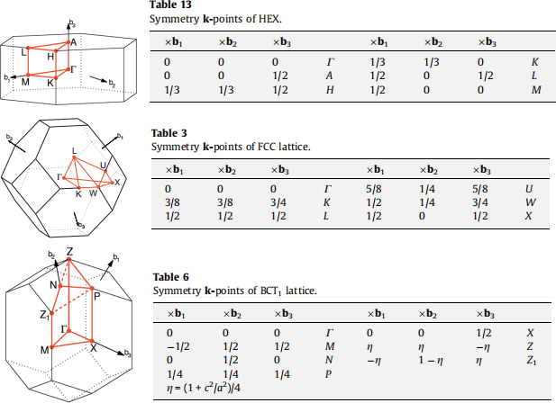
Figure 1: Brillouin  zone  (left)  and  special  points  coordinates  (right)  of  a  hexagonal (top), face-centered cubic (middle), and body-centered tetragonal Bravais lat- tice (bottom). From Comp. Mat. Sci. 49, 299-312 (2010).