GGR201H5S Winter 2024 Practical Exercise 1 (Weeks 1-4): Topographic maps and glacial landforms Part i
Hello, dear friend, you can consult us at any time if you have any questions, add WeChat: daixieit
GGR201H5S
Winter 2024
Practical Exercise 1 (Weeks 1-4): Topographic maps and glacial landforms
Part (i): Analysis of topographic maps and introduction to virtual fieldwork
Due: Monday 5th February, 9 pm
Outline & rubric
|
Practical class |
Assignment component |
Mark |
|
January 12th |
Part (i) Analysis of Topographic Maps / Glacial Landscapes (virtual fieldwork) Section 1 – interpreting contour maps Section 2 – constructing topographic profiles Section 3 – virtual fieldwork |
6 14 20 |
|
January 19th |
Part (ii) Landscapes of glacial retreat - the Tschierva Glacier, Switzerland Section 4a – topographic profiles Section 4b – glacial landforms Section 5 – timescales of glacier retreat |
20 10 5 |
|
January 26th |
Part (iii) Glacial landforms in the Peterborough area of Southern Ontario. Section 6 – topographic profiles Section 7 – glacial landforms |
15 30 |
|
February 2nd |
Parts (i-iii) (continued) Online submission by 5th February, 9 pm |
|
|
|
Total: |
120 |
Introduction to Practical 1
Practical Exercise 1 is in three parts, beginning with an introductory exercise (Parti) on Friday 12th January and continuing with explorations of glacier retreat in the Tschierva Glacier, Switzerland (Part ii) and glacial landforms in the Peterborough area of Southern Ontario (Part iii). See table above for details of the content and rubric. A common theme throughout Practical 1 is the observation and analysis of landforms and landscapes associated with recent historic glacier retreat in both mountainous and low-relief landscapes.
All three parts of Practical 1 take the form of weekly self-guided worksheets that can be completed in your own time; the timetabled Practical classes will be used to illustrate key techniques and approaches and to offer support and guidance for the respective tasks. Aspects of glacial erosion, deposition and landform development will also be covered in Lectures 2-4 in advance of the Practical submission (Parts i-iii) on 5th February.
Part (i) Analysis of Topographic Maps and introduction to virtual fieldwork
Part (i) begins with a modified version of exercises developed by Christopherson and Thomsen (2009) and focuses on a key diagnostic tool for landform analysis - the topographic map. Sections 1 and 2 are intended to familiarize you with the use of topographic maps in a geomorphological context and as a tool for interpreting and mapping landforms. A core aspect of this practical is an appreciation of isolines, or lines that connect points of equal value – on topographic maps these are called contour lines and they connect points of equal elevation.
Section 3 of the practical will introduce you to a virtual fieldtrip website (VR Glaciers and Glaciated Landscapes) in order to explore and describe a series of geomorphological features in the Roseg Valley, Switzerland, an alpine glacial landscape which hosts the Tschierva Glacier. Although this part of the practical precedes the glacial geomorphology part of the Lecture series, you will have time to revise and refine your work before the submission.
Objectives
After completion of this practical you should be able to:
1. Interpret contour lines (isolines of equal elevation) on topographic maps;
2. Construct a topographic profile and calculate an appropriate vertical exaggeration for a profile;
3. Use virtual fieldwork resources to generate and annotate images of specific landforms associated with glaciated landscapes.
Instructions
Read each section below and complete the exercises and written questions in the spaces provided – note that the topographic profile exercises are best undertaken by hand-drawing on printed hardcopy, and that submission of the practical will requirescanned or photographed copies of your completed drawings. Submission instructions will be provided in Part (iii) of the Practical.
Resources
Sections 1 and 2
The following video guides on Youtube provide useful introductions to interpreting contours and drawing topographic profiles (you’ll recognize one of the examples in the first video) –
recommended if you have no experience in these techniques:
• Introduction to Topographic Maps:https://www.youtube.com/watch?v=zqPMYGDxCr0
• Topographic Profiles:https://www.youtube.com/watch?v=KhlhkgYoeOQ
Section 3
Before starting Section 3 it is recommended that you take the time to familiarize yourself with VR Glaciers and Glaciated Landscapes (https://vrglaciers.wp.worc.ac.uk/wordpress/). This has a similar functionality to Google Streetview, but has been developed to support geomorphological exploration (via virtual fieldwork) of past and present glaciated landscapes. You’ll find a useful video introduction on the site homepage (link also here:https://youtu.be/DDMP23vJ7sI).
Further aspects of the site will be explored in the Practical session.
Section 1: Interpreting contours
Topographic maps portray physical relief (the change in elevation between the highest point and lowest point on the map). Relief is indicated through the use of elevation contours – lines that connect all points at the same elevation above or below a stated reference level. This reference level (usually mean sea level) is called the vertical datum. The contour interval is the difference in elevation between two adjacent contour lines. In Figure 1 the contour interval is 20 ft.
The topographic map in Figure 1 shows ahypothetical landscape that demonstrateshow contour lines and intervals depict slope and relief. Slope is indicated by the pattern of contours and the space between them. The steeper a slope or cliff, the closer together the contour lines appear (compare the contour line spacing between the cliffs and beach area on Figure 1). You should also see that contour lines crossing stream valleys form a V pointing upstream. Finally, note the presence of a spot height marked with an ‘x’ and elevation label.
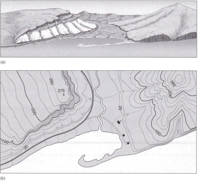
Figure 1: (a) Perspective view of a hypothetical landscape; (b) topographic map of that landscape
Section 1 exercise: (6 marks, 1 per question)
Use the hypothetical landscape and topographic map in Figure 1 to answer the following questions:
a) What is the contour interval?
b) How can you tell?
c) In terms of the local relief (the difference between the highest and the lowest elevation):
(i) what is the relief on the west (left) side of the road?
(ii) on the east (right) side of the road?
d) What is the highest point on the map and what is its elevation?
e) Figure 1 also shows a river and several smaller streams; how do the contour lines indicate the direction of flow?
Section 2 - constructing topographic profiles
Figure 2 demonstrates the technique for constructing a topographic profile (a graphic representation of graduated elevationsalonga line segment drawn on a map) from contour data; the profile reflects elevation changes along a line connecting two points (atransect). Topographic profiles complement map views (i.e. bird’s-eye views) of a landscape by revealing the shape of the land as viewed from the side.
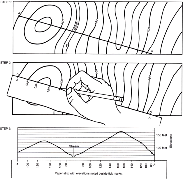
Figure 2: Constructing a topographic profile using the edge of a piece of paper
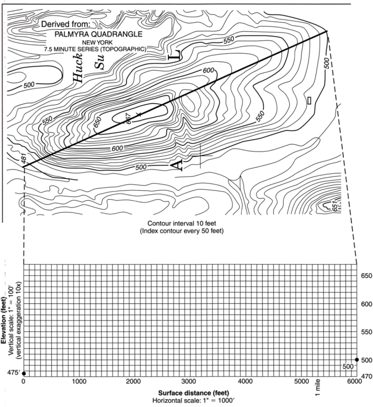
Figure 3: Topographic profile from the Palmyra, New York map quadrangle (enlarged)
Section 2 exercise: (14 marks: 9 for the profile, 5 for questions)
Construct a topographic profile using Figure 3; this portrays an area near Palmyra, New York, a region that was overrun by continental glaciers during the last glaciation. The feature being profiled was deposited by a glacier. A prepared graph is provided with the figure - note that this graph employs a vertical exaggeration technique to convey a better impression of the landform profile. The map in Figure 4.6 has a horizontal scale of 1:12,000 (or 1 inch = 1000 ft); if we used this same scale for the vertical axis on the topographic profile graph the local relief of 192 feet would only cover 0.192 inch on the graph. To construct a readable and useful profile the graph uses a vertical scale of 1:200 (or 1 inch = 100 ft) which represents a 10x exaggeration of the horizontal scale. Other landscapes may require different vertical exaggeration – in general, the greater the maximum relief of a landscape, the greater the greater the scale should be to conveniently fit on a graph for analysis.
Follow the procedure illustrated in Figure 2 to construct a profile along the transect shown in Figure 3, making tick marks on your paper at each point where the drawn line and contour lines intersect. Carry the elevations denoted by the tick marks down to the graph, plotting each point. The steeper the slope the closer the points are placed: a gentle slope places them farther apart. The last step is to connect the points with a smooth curved line to visualize the relief and topography of the landscape. You may want to shade the area below the line to better display the profile.
Use the profile constructed in Figure 4 to answer the following:
a) What distance does this topographic profile cover?
b) What is the maximum relief along this profile?
c) The landform feature you have profiled is a drumlin. Drumlins are formed by glacial deposition and are streamlined in the direction of the glacier’s movement. They have a blunt end upstream, a tapered end downstream and a rounded summit. Draw an arrow above your topographic profile to indicate ice-flow direction implied by the drumlin profile.
d) Using the 500-foot (or nearest) contour, what is the approximate width of this feature at its widest?
e) If we used a vertical scale identical to the horizontal scale, how many squares on the graph would accommodate the maximum relief along the profile?
Section 3 - Glacial Landscapes (virtual fieldwork) (20 marks - 2 for each feature)
Navigate to The Roseg Valley Virtual Fieldtrip:
https://vrglaciers.wp.worc.ac.uk/wordpress/roseg-valley-virtual-field-trip/
Once on the web page scroll down and click ‘Take me there’. Take the time to explore the landscape and features of the valley, especially from the viewpoints near the snout of the Tschierva Glacier and the valley below (viewpoints 6-9 and 11-14).
a) Using the viewpoints provided in the VR fieldtrip, identify what you consider to be a good
example of each of the landform features listed below. You may find Fig. 7.11 from Trenhaile (2016) useful here – see below.
b) Take a screenshot (or use an application such as Snipping Tool) of each feature, noting that
you can zoominor out to obtain a good composition, and paste it into the appropriate section in the listing below. Images should betaken from the main (left-hand) VR window, although some features may also benefit from supplementary images from the right-hand map (satellite) pane if you wish (especially horn / arête).
c) Use the basic drawing tools in Word to label or annotate the feature (e.g.
Insert/Shapes/Lines/Line arrow) so that it is clear which landform you are describing. Note – you might find it easier to use Powerpoint for graphic annotation, etc. You can then screenshot or clip the annotated image and paste into Word.
d) In the space below each image provide a short (c.50 words) description of the feature and justify your interpretation (e.g. on the basis of shape, location, etc). See below for example image and information.
Landform features:
1. Cirque glacier
2. Arête
3. Horn
4. Glacier snout (Tschierva Glacier)
5. Glacial trough (U-shaped valley)
6a & b. Lateral moraine (two examples)
7. Scree / talus
8. Valley train
9. Ground moraine
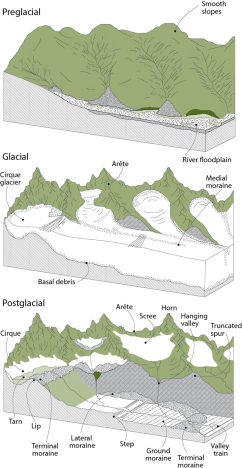 Trenhaile (2016) Fig 7.11
2024-02-03
Analysis of topographic maps and introduction to virtual fieldwork