Multivariable Design Coursework An Introduction to H∞ Design
Hello, dear friend, you can consult us at any time if you have any questions, add WeChat: daixieit
Multivariable Design Coursework
An Introduction to H∞ Design
1 Introduction
The aim of the coursework is to introduce you to H1 control sys- tem design. All the background material you may need is found in the Robust Control Toolbox. You should read Section 3 in the tutorial section before attempting any part of the coursework. The theoretical work can be found in the lectures on multivariable control.
2 A lightly damped beam example
The purpose of the section is to introduce you to the siso mixed sensitivity problem (see the Robust Control Toolbox for a precise deinition). The plant considered is contrived to illustrate various features of the H∞ theory, but is vaguely reminiscent of a lightly damped beam with its sensors and actuators
The design will be carried out in a number of steps:
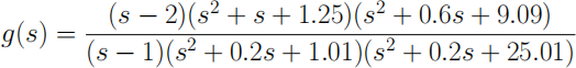
1. Use the conv command to input the plant model into the vari- ables num and den in matlab; we want g(s) = num/den.
2. Find a state-space model for g(s) using the command tf2ss.
3. Find the poles and zeros of g(s) using the commands eig and tzero respectively.
4. Plot a frequency response of g(s) using the command sequence:
. ω = logspace(-2,3,150);
. mag = bode(num,den,w);
. semilogx(ω, 20 * log10 (mag))
and reconcile this plot with the poles and zeros of g(s) (i.e. identifying the poles and zeros by looking at the shape of the bode plot such as the asymptotes).
5. We will now design a controller for the sensitivity alone; we want a good tracking property over the frequency range 0-5 rad/s. To this end we solve the problem

or equivalently,

where,
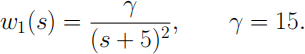
6. Embed this design in a larger problem as follows. Let,
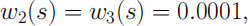
and form,
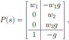
using the augment command as follows: (create your own .m ile containing this),
. Gam = 15;
. dnw1i = 1; nuw1i = [1, 10, 25];
. dnw1 = [1, 10, 25]; nuw1 = 1;
. dnw2 = 1; nuw2 = 0.0001;
. dnw2i = nuw2; nuw2i = dnw2;
. dnw3 = 1; nuw3 = 0.0001;
. dnw3i = nuw3; nuw3i = dnw3;
. [aw1, bw1, cw1, dw1] = tf2ss(dnw1i * Gam,nuw1i);
. sysg = [ag, bg; cg, dg]; sysw1 = [aw1, bw1; cw1, dw1];
. [rdg, cdg] = size(dg);
. sysw2 = [0.0001]; sysw3 = [0.0001];
. dim = [5, 2, 0, 0];
. [A, B1, B2, C1, C2, D11, D12, D21, D22]
= augment(sysg, sysw1, sysw2, sysw3, dim);
7. Calculate an H1 controller using the command hinf syn.
8. Plot W![]() 1 (s), W3-1 (s), the sensitivity and the complemen- tary sensitivity by typing the command pltopt in the com- mand window. The value of is user-deined and in this case = 15. Follow the steps shown in the command window.
1 (s), W3-1 (s), the sensitivity and the complemen- tary sensitivity by typing the command pltopt in the com- mand window. The value of is user-deined and in this case = 15. Follow the steps shown in the command window.
Alternatively, you can open the relevant m–ile by typing in open pltopt.min the command window. Be aware that the pa- rameters ag, bg, cg, dg, nuw1i,dnw1i,nuw3i,dnw3i are the inputs of this m–ile and they need to be speciied beforehand. Analyse the plots and comment on the loop tracking properties of the design.
9. Find the closed-loop poles and check they are stable. Find the controller poles and zeros and explain what the controller is doing to the stable and minimum phase factor of the plant.
10. Suppose the (s-2) term in the numerator of g(s) were replaced by (s + 2). How big could we make and why?
11. Interpret the complementary sensitivity as a robustness mea- sure and comment on the robustness of the above design. Would you be happy with this design from a robustness point of view? (Ignore step (10)).
12. Suppose we want the complementary sensitivity smaller than
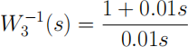
for robustness reasons. Introduce this W3 and let = 11 in
the weight W1 (s) above.
13. Find the new augmented plant as above and repeat the design calculation using hinf syn.
14. Plot W![]() 1 (s) and W3-1 (s). Compare the robust stability prop- erties of the old and new designs. Are there any improvements? Explain the trade made between performance and robustness.
1 (s) and W3-1 (s). Compare the robust stability prop- erties of the old and new designs. Are there any improvements? Explain the trade made between performance and robustness.
15. Use Simulink to validate the tracking abilities of both de- signs above by performing time responses (i.e. step or pulse responses). Explain your indings.
3 A 1990’s aircraft example
In this experiment we consider the longitudinal dynamics of the HI- MAT experimental aircraft trimmed at an altitude of 25,000ft and a speed of 0.9 Mach. The control variables are the elevon and canard actuators, while the output variables are the angles of attack and attitude. See the tutorial section of the Robust Control Toolbox for further details. Obtain the aircraft model by running hinfdemo and using Option 2. Alternatively make a copy of the Matlab ile hmatdemo.m which you can change to perform the remainder of the experiment. This can be done by typing in open hmatdemo.m in the command window.
Preliminary analysis
Calculate the open-loop poles and zeros, plot the frequency re- sponse and comment on the expected difficulties associated with synthesising a control system for such a plant. Explain your an- swer.
The design speciications
1. The robustness speciication requires that the complementary sensitivity function rolls of at -40db per decade over frequen- cies beyond 100 rad/s and that it is no greater than -20db at 100 rad/s. Design a weighting function that meets these speciications without imposing any extra conditions at low frequencies.
2. With the above robustness speciications in mind, we require that the sensitivity is as small as possible between 0 and 1 rad/s.
The controller design and analysis phase
1. Choose weighting matrices W1(s) and W3(s) which reflect the design specifications on performance and robustness, respec-tively. Remember that W2(s) must be set equal to some small full rank constant matrix. Explain why this is necessary. Ex-plain how you would synthesise the improper weighting func-tion W3(s). Follow step (6) of the first design to augment the plant.
2. Calculate your own controller using the hinfsyn command; all the standard plots may be obtained using the command pltopt as before. Interpret the robustness and sensitivity char-acteristics of this design.
3. Plot W1 −1 (s), W3 −1 (s), the sensitivity and the complementary sensitivity functions. Tune the value of γ to obtain the best possible design which meets the specifications.
4. Plot ¯σ[K(I + GK) −1 ]. In the light of this plot, is this control system implementable? Carefully explain your answer and back up your comments with appropriate graphs. Indicate how this situation may be remedied and do so.
5. Interpret ¯σ[K(I + GK) −1 ] as a robustness indicator by com-paring the sizes of the perturbations that might be accommo-dated in the two designs (i.e. step (3) and step (4)). Indicate how the two designs are changed and what trade–offs have been made.
6. Compare the time responses of the near optimal design of step (3) with those of the near optimal design of step (4).
2024-01-29