ECON 178 WI 2024: Homework 1
Hello, dear friend, you can consult us at any time if you have any questions, add WeChat: daixieit
ECON 178 WI 2024: Homework 1
Due: Feb 6, 2024 (by 2:00pm PT)
Instructions:
• The homework has a total of 40 points. The TAs will randomly pick one problem to grade and this problem is worth 30 points (you will get 30 points if your answers are correct or almost correct). The remaining 10 points will be graded on completion of this assignment.
• There will be two separate submissions: one for your R code and one for your writeup. Please submit both on Gradescope (more details for the submission of the R part are given in “Applied questions”).
• Every student in ECON178 must read, understand, agree and sign the integrity pledge (which is posted under Modules on Canvas) before completing any assignment for ECON178. Please include your signed pledge in the submission of your assignment on Gradescope.
Conceptual questions
The following questions involve reviewing exercises about expectations, conditional expectations, biases and variances, and basic properties of Normal (also called Gaussian) distributions.
Question 1
![]() Suppose that we have a model yi = βxi+ ei (i = 1, ..., n) where y
Suppose that we have a model yi = βxi+ ei (i = 1, ..., n) where y![]() =
= ![]() Σ
Σ![]() , x =
, x = ![]() Σ
Σ![]() = 0, and ei is distributed normally with mean 0 and variance σ2 ; that is, ei ∼ N (0, σ2 ). Furthermore, e1 , e2 , ..., en are independently distributed, and the x is (i = 1, ..., n) are non-random.
= 0, and ei is distributed normally with mean 0 and variance σ2 ; that is, ei ∼ N (0, σ2 ). Furthermore, e1 , e2 , ..., en are independently distributed, and the x is (i = 1, ..., n) are non-random.
(a) The OLS estimator for β minimizes the Sum of Squared Residuals:
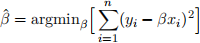
Take the first-order condition to show that
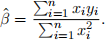
(b) Assume E [ei|β] = 0 for all i = 1, ..., n. Show that
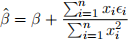
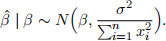
What is E[β(ˆ) | β] and Var(β(ˆ) | β)? Use this to show that, conditional on β , β(ˆ) has the following distribution:
(c) Suppose we believe that β is distributed normally with mean 0 and variance ![]() ; that is,
; that is,
![]() β ∼ N (0,
β ∼ N (0, ![]() ). Additionally assume that β is independent of ei for all i = 1, ..., n. Compute
). Additionally assume that β is independent of ei for all i = 1, ..., n. Compute
(Hint you might find useful: E[w1] = E[E[w1 | w2]] and Var(w1 ) = E[Var(w1 | w2 )] + Var(E[w1 | w2]) for any random variables w1 and w2.)
(d) Since everything is normally distributed, it turns out that
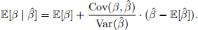
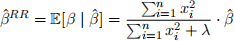
Let β(ˆ)RR = E[β |β(ˆ)]. Compute Cov(β,β(ˆ)) and use the value of E[β] along with the values of E[β(ˆ)], Cov(β,β(ˆ)), and Var(β(ˆ)) you have computed to show that
(Hint: Cov(w1 , w2 ) = E[(w1 − E[w1])(w2 − E[w2])] and E[w1w2] = E[w1E[w2 | w1]] for any random variables w1 and w2 )
(e) Does β(ˆ)RR increase or decrease as λ increases? How does this relate to β being distributed N (0, ![]() )?
)?
Question 2
Let us consider the linear regression model yi = β0 + β1xi + ui (i = 1, ..., n), which satisfies
Assumptions MLR.1 through MLR.5 (see Slide 7 in “Linear_regression_review” under “Modules” on Canvas). The xis (i = 1, ..., n) and β0 and β1 are nonrandom. The randomness comes from uis (i = 1, ..., n) where var (ui) = σ2 . Let β(ˆ)0 and β(ˆ)1 be the usual OLS estimators (which are unbiased for
β0 and β1 , respectively) obtained from running a regression of  (the intercept column) and
  . Suppose you also run a regression of
  only (excluding the intercept column) to obtain another estimator β(˜)1 of β1 .
a) Give the expression of β1 as a function of y is and x is (i = 1, ..., n).
b) Derive E (β(˜)1 ) in terms of β0 , β1 , and xis. Show that β(˜)1 is unbiased for β1 when β0 = 0. If
β0 ![]() 0, when will β1 be unbiased for β1?
0, when will β1 be unbiased for β1?
c) Derive Var (β(˜)1 ), the variance of β(˜)1 , in terms of σ2 and x is (i = 1, ..., n).
d) Show that Var (β(˜)1 ) is no greater than Var (β(ˆ)1); that is, Var (β(˜)1 ) ≤ Var (β(ˆ)1). When do
you have Var (β(˜)1 )= Var (β(ˆ)1)? (Hint you might find useful: useΣ![]() xi(2) ≥Σ
xi(2) ≥Σ![]() − x(¯))2 where
− x(¯))2 where
![]() e) Choosing between β(ˆ)1 and β(˜)1 leads to a tradeoff between the bias and variance. Comment on this tradeoff.
e) Choosing between β(ˆ)1 and β(˜)1 leads to a tradeoff between the bias and variance. Comment on this tradeoff.
Applied questions (with the use of R)
For this question you will be asked to use tools from R for coding.
Installation
• To install R, please see https://www.r-project.org/.
• Once you install R, please install also R Studio https://rstudio.com/products/rstudio/ download/.
• You will need to use R Studio to solve the problem set.
Download
from Canvas ⇒ Assignments
• data_ps1.csv;
• template_ps1.R .
Submission
• Open the template_ps1.R file that we provided on Canvas ⇒ Assignments.
• All your solutions and code need to be saved in a single file named
template_ps1_YOURFIRSTANDLASTNAME.R file. Please use the template_ps1.R pro- vided in Canvas to structure your answers.
• Any file that is not an .R will not be accepted, and the grade for this exercise will be zero.
• Please submit your code on Gradescope.
• Please follow the policy stated in the syllabus about academic integrity.
Useful readings
In addition to the lectures provided by the instructor and the TAs, you might find the following readings useful:
• Chapter 2.3 and 3.6 in the textbook ”An introduction to statistical learning with applications in R”.
Question 3
This exercise helps you get familiar with basic commands in R by working with the Forest Fires data set (Dua, D. and Graff, C., 2019, UCI Machine Learning Repository;2 see:
https://archive.ics.uci.edu/ml/datasets/Forest+Fires). This data set is available on Canvas ⇒ Assignments.
1. Download the dataset from Canvas and open it using the command “read.csv”.
2. Open the data and report how many columns and rows the dataset has;
3. See the names of the variables (see online the command “names”);
4. Run a linear regression with “area” as a function of “temp” using the command “lm”;
5. Report the summary of your results (see online the command “summary”)
7. Plot a scatter plot of the regression (Hint: use abline() to draw the regression line)
8. Write down the interpretation of the coefficients as a comment in your .R script (Hint: see template file).
Please write all your answer and code in template_ps1.R file and submit that file on Gradescope as described in the “Submission” section.
2024-01-27