Hello, dear friend, you can consult us at any time if you have any questions, add WeChat: daixieit

PPHA311

ProblemSet3

Winter2024

1 The Oregon Health Insurance Experiment, Revisited (16 points)

In this problem, you will continue to work with the data from Problem Set #1, Q2. Please refer back to Problem Set 1 for variable definitions.

For this assignment, you can refer to any output that comes from the lm() function in R.

1. 

In Problem Set Q2.1, we found that one of the baseline characteristics, numhh list, was statistically significant from zero at the 5 percent level. Oh no, did randomization fail? It turns out that the researchers expected this. The reason this happened is because treatment was assigned at the household level, and households with more eligible individuals had more chances to win the lottery. Fortunately, we can easily deal with this violation of balance using multivariate regression techniques!

The regression controlling for family size is given as follows:

 (2)

For each of the five outcomes, calculate the bias from not including numhh list as a control, filling in the table below. Are any of these biases quantitatively large enough to fundamentally change any of your qualitative conclusions about the OHIE? (3 points)

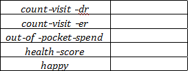
2. Let’s look at which groups increased their doctor office visits the most in response to the treatment. Fill in the table below by running separate regressions of visit dr on treated, and controlling for numhh list, i.e. by running model (1) above, for each of the groups listed in the table. Discuss your findings: which group has the largest estimated treatment effects, which group has the smallest? Be sure to also consider the statistical significance. (3 points)

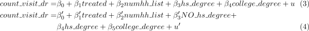
3. Returning to the full data and still focusing on the number of doctor office visits, let’s also try controlling for education.

Using information in the variables hs degree and college degree, create a new indicator variable if someone DOES NOT have a high-school degree, call this new variable NO hs degree.

Try running each of the following regressions. Discuss how your estimated treatment effect, the precision of this estimate (standard error), and R² changes from just including numhh list, i.e. model (1) above. If you cannot estimate a coefficient, explain why. (3 points)

4. Now, let’s try including all the baseline characteristics as controls to the regression. Rerun the regression of count_visit_dr on treated, and control for:

numhh_list, female, age, race_white, hs_degree, college_degree, health_baseline

How does your estimated treatment effect, the precision of this estimate (standard error), and R² change from the model just including numhh list (2 points)

5. Do you think we should include all these other baseline characteristics as controls to ensure that the treatment effects are unbiased, or is it sufficient to just control for numhh list? Explain. (1 point)

6. Do you think we should include all these other the baseline characteristics as controls to improve the precision of our estimated treatment effects? Explain. (1 point)

7. Using the model with the full set of controls estimated in Question 4, conduct a hypothesis test that the treatment effect on the number of doctor office visits is equal to the effect of having a high school degree.

Note: In class on Jan 23, we discussed two different ways to conduct this test. You can choose either method.

To receive full credit, you should code this test manually in the manner we discussed in class and not use the anova() function or other such functions to perform hypothesis testing. (3 points)