1    Purpose

This assignment should give you some hands-on experience with designing and implementing discrete time (“digi- tal”) systems, and apply them to filtering audio signals.

The assignment will contribute 10% to your overall mark in EE320.

2    Completion, Submission, and Assessment

Please submit your assignment via MyPlace by Monday 5/2/2023, noon. Your submission should include

1.  an m-file containing your implementations and generating any plots;

2.  a brief document containing your answers and any supporting graphs; this does  not have to be a formal report — answers should be brief, but justifications  are  important,  and  any  supporting evidence  (matlab plots, calculations / references to material covered in the lectures) should be included. Scans or photographs of your handwritten workings are perfectly acceptable.

You can receive assistance with your assignment during a number of surgeries which we will hold during December 2023 and January 2024.  These will be typically Tuesdays 9-11am in R446.  Detaiils be announced separately via MyPlace.

We will assess your solution based on the correctness of your implementations, and the justifications that you have provided.  We may hold interviews to assess your understanding and to ensure that the submitted work is yours; in this case an interview will contribute to or overwrite the assessment of your submission.  Therefore, you should only submit what is your own work, and be sure that you understand its purpose.

If you wish to work on this problem during the University holidays and do not have access to Matlab, you can consider the free Matlab clone Octave (https://www.gnu.org/software/octave/) which can do almost everything possibly except for playing audio files.

Important:  this exercise involves audio files.  If you listen to any audio files, particularly when using headphones, please ensure that you select a low volume, in case the signal amplitude is high!

3    Problem

Two ears / microphones pick up signals x1 [n] and x2 [n], which are a mix of two speakers and a sinusoidal inter- ference.  The two speakers are active concurrently  (“cocktail party effect”), and the aim will be to retrieve their signals individually and without the interference. The solution will be based on temporal and spatial filtering.

The situation is illustrated in Fig. 1. We assume two microphones that are separated by d = 17.15cm, mimicking the distance between the two ears of an average (or at least weiss-sized) head. As sources, two speakers si [n], i = 1, 2, simultaneously speak; we assume that these speakers are in the far-field and that the propagation is free-space, i.e. there are no reverberations or echos, and the speakers’ signals arrive as planar wavefronts at the microphones. The impulse response between a source si [n] and the microphone signal xm [n] therefore will only be a delay and gain factor. Additionally, there is a sinusoidal interferer present, which corrupts the two microphone signals xm [n], m = 1, 2.  Overall, we have

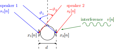
Fig.  1:  Scenario with two speakers and sinusoidal  interference at two microphone mimicking the positions of ears on a head.

where τj , i = 1, 2, are delays and ρm,i  and ρm,v , m, i = 1, 2 are gain factors.

We are only interested in the relative delay and gain that a source experiences across the two microphone signals. For example, if we were only to receive a single signal, say s1 [n], then for the two microphone signals xm [n], we have

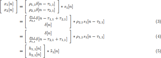
We want to work with positive delays, such that a delay function R1 δ[n — T1] is causal and has a gain R1  < 1. For ϑ1  > 0, the path to x2 [n] will have a longer delay, and hence a greater attenuation, and (3) applies.  In the case ϑ1  < 0, we select representation (4).  The general model in (5) ties this to impulse responses hm,1[n], where Hm,1(z) .—O hm,1[n] are known as relative transfer functions.  We would like to recover the potentially shifted and attenuated source signal ˜(s)1 [n].

We can then create an inverse matrix G(z) = H −1 (z).  Such an inverse does not always exist, but is possible for

our parameter range, and detailed in Appendix A. With G[n] O—. G(z), we can the create two outputs ym(′)[n], m = 1, 2,

in which the speakers should appear separated. The design of this filter G[n] is detailed in Fig. 2.

The separated signals ym(′) [n] are still subject to sinusoidal interference. To remove this interference, the aim is

to construct a bandstop filter Q(z) that is capable to suppressing this noise component while preserving the speech

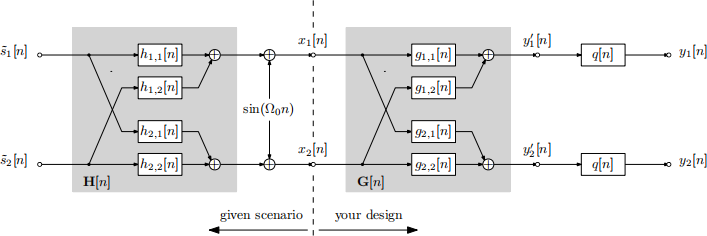
Fig. 2:  Scenario with two speakers and sinusoidal interference captured by two microphone signals x1 [n] and x2 [n].  The schematic shows the processing that you are expected to implement in order to separate the source signals and to suppress the interference, based on an analysis of the paths hm,i [n] and the interfernece frequency Ω0 . signal as best as possible.  The outputs ym [n] from this filtering operation in Fig. 2 should ideally sound close to the separated, noise-free speech signals ˜(s)m [n], m = 1, 2.

4    Precursor

In Matlab, you can read in and play audio files, including stereo ones.  To appreciate the spatial impression that you can get from stereo channels, feel free to try the following:

u1 = audioread(’speaker1.wav’);        % read in a single channel signal

u2 = filter([0 0 1],1,u1);                       % delay by two sampling periods

f2 = 8000;                                         % sampling frequency in Hertz

sound([u1 u2],fs);                             % play back stereo

The sound should appear to come slightly from one side. If you are unconvinced of the directionality, play

sound([u2 u1],fs);                % reverse stereo channels

This should sound different — the source should now appear to be on the other side.

5    Scenario and Analysis

Based on your student registration number, StudRegNum, as a parameter, you can obtain the signals x1 [n] and x2 [n] as the output of the function

[x1,x2] = AssignmentScenario(StudRegNum);

Please ensure that you have downloaded the files speaker1.wav and speaker2.wav, and that they are visible from your Matlab working directory.  These files contain your source signals  si [n], i = 1, 2, and these files need to be read by the function AssignmentScenario().  If you listen to one output via e.g. sound(x1,8000), you should hear a mix of two speakers and a tone.

5.1    Analysis of Sinusoidal Interference

For later interference cancellation, we require a good estimate of the interference frequency — you are asked to perform this in both the time and frequency domains.

Question 1 (Time domain analysis of interference frequency.)  Estimate  the  frequency  f0    or  normalised angular frequency  Ω0   =  2πf0 /fs   of  the  interferer  by  inspecting  the  time  domain  waveform  x1 [n] .     This  is   best over a  segment  of the  signal  where  the  speakers  are  otherwise  quiet  (i.e.  interference  dominates),  such  as  during the first couple  of hundred samples  of x1 [n] .

Question 2 (Frequency domain analysis of interference frequency.)  Estimate  the  interference  frequency by evaluating the  discrete-time Fourier transform

fs = 8000;                                              % sampling frequency in Hertz

f = (0:length(x1)-1)/length(x1)*fs;        % frequency scale

plot(f,abs(fft(x1)));                                 % discrete Fourier transform of x

xlabel(’frequency f / [Hz]’);                    % label axes

ylabel(’magnitude’);

Question 5 (Delay and gain estimation in the Fourier domain.)  For a signal consisting of N samples, com- mand fft() approximates  (closely  enough for  our purposes)  the  Fourier  coefficients  of the  discrete  time  Fourier   transform at a Nof isolated,  equispaced frequency points  between DC and the  sampling frequency.  For  example,

fs = 8000;                                         % sampling frequency in Hertz 

Range = (19501:21548);                   % window of samples to investigate

N = length(Range);                      % number of samples

X1 = fft(x1(Range));                    % Fourier coefficients via fft()

f = (0:(N-1))/N*fs;                       % frequency scale

plot(f,abs(X1));                              % plot magnitude of coefficient

xlabel(’frequency f / [Hz]’);               % label axes

ylabel(’magnitude’);

Question 12 (Filter sequence.)  Very briefly justify whether or not it is possible to swap the notch filters Q(z) with the unmixing system  G(z) .

8    Final Comments

This assignment uses your signals and systems tools to take you beyond applications that you have encountered in the lectures. Please engage during the surgery / Q&A sessions to ensure that you have understood the task in all its aspects, and feel free to discuss your approach.  You may find it interesting that the topic of this assignment takes you to the cutting edge of research, where relative transfer functions are making an impact in the audio word, and matrices of transfer functions are a generic way of describing and solving signals & systems problems.

A    Appendix:  Inverting a Matrix of Transfer Functions

For a standard 2 × 2 matrix, its inverse can be easily found as

as long as the determinant satisfies ad − bc  0.

For  a  matrix  H (z)  of transfer  functions  as  in  (6),  as  long  as  the  determinant  D(z)  =  H1 , 1 (z)H2 ,2 (z) − H2 , 1 (z)H1 ,2 (z) does not possess any zeros on the unit circle, we have

Example: For H (z) with H1 , 1 (z) = H2 ,2 (z) = 1, H1 ,2  = ρz −2  and H2 , 1  = ρz −1, the inverse  G(z) is

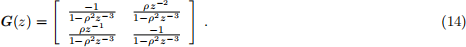
The implementation could use the filter() command in Matlab, such that for inputs yprime1 and yprime2 and some defined factor rho with a modulus smaller than one, the outputs are

y1 = filter(-1,[1 0 0 -rho^2],yprime1)                     + filter([0 0 rho],[1 0 0 -rho^2],yprime2);

y2 = filter([0 -rho],[1 0 0 -rho^2],yprime1)               + filter(-1,[1 0 0 -rho^2],yprime2);