There will be three multi-part questions:

•      one on Decision Trees

•      one on Monte Carlo Simulation

•      one on Optimization

There are some parts that can be answered without the computer, but most parts will require the construction and solution of an appropriate spreadsheet model. You will need to use TreePlan, Crystal Ball, and Solver on the exam. You will not need to use SensIt (the tornado chart tool).

1) Decision Tree Skills

a)  Constructing a tree from a verbal description of the problem: capturing the sequence of decisions, uncertainties, and cash flows.

b) Rolling back the tree: Calculating expected values at uncertainty nodes and selecting the best value at decision nodes. You will be using TreePlan, so you won’t have to do the calculations by hand, but make sure you understand them.

c)  Sensitivity analysis: How do the outputs of the model (optimal strategies and expected values) change when you change an input (a probability or a cash flow)? This can be done by hand algebraically or in Excel with a Data Table or using Goal Seek.

d) Calculating the value of information:  How much value is there to having an uncertainty fully or partially resolved before you have to make a choice? To find the expected value of the information, draw a new tree reflecting the new sequence in which decisions and uncertainties occur, and look at the increase in expected value in the new tree compared to the original tree. Information has value if and only if it changes some decision.

i)  Perfect information: To calculate the expected value of perfect information (EVPI), redraw the tree to have the uncertainty in question before the decision(s), and find the increase in expected value compared to the original tree which has the uncertainty resolved after the decision.

ii) Imperfect (or Sample) information: To calculate the expected value of sample information (EVSI), the outcome of an imperfect testis revealed before you have to make your decision.

e)  Incorporating risk preferences into a decision tree by using an exponential utility  function. Calculating certainty equivalents by computing rollback values in terms of expected utility, and applying the inverse utility function to these expected utilities. Recall that the exponential utility function with risk tolerance R is given by

u(x) = 1 − exp (−x/R)

and the corresponding certainty equivalent (inverse utility function) is given by

CE(EU) = −R ∗ ln(1 − EU).

f)  Evaluating different strategies (a pre-specified decision policy) in a decision tree by comparing the cumulative risk profiles that they induce. Using our definitions of “stochastic dominance” (one cumulative risk profile is always to the right or

left of the other) and “riskiness” (the cumulative risk profiles cross exactly once, with the less risky strategy being the “steeper” curve and the more risky strategy being the “flatter” curve) ordering to make these comparisons, if such an ordering exists. Note that if one strategy is less risky and has a better expected value, then  it will be preferred by any risk-averse or risk-neutral decision maker (which in practice is essentially everyone).

2) Monte Carlo Simulation Skills

a)  Building a deterministic model from a description of the situation. That means building a spreadsheet model that takes values in input cells and computes outputs (i.e., the objective, any subtotals needed to compute the objective, other quantities of interest). Some inputs may actually be uncertain, some maybe decision variables, but at this point they are all treated as fixed numbers.

b)  Selecting appropriate probability distributions for key uncertainties (CB “assumptions”). Some considerations to guide your thinking:

i)  Is there a theoretical structure that calls for the use of a particular distribution? (For example, a binomial random variable represents the number of successes out of n independent events, each with probability of success p.)

ii) What are the properties of the uncertainty you are trying to model (e.g., discrete or continuous, bounded above or below or both, symmetric or asymmetric)?

iii) Is there data from which to build or fit a distribution?

iv) Do you have expert assessments of some of the characteristics of the distribution (e.g., 10th-50th-90th percentiles)?

v) Are the random quantities independent? If not, can I express the dependence through a relationship between the draws from one distribution and the parameters of another, or can I express it as a correlation?

c)  Selecting outputs to track (CB “forecasts”).

d) Considering a range of values for a decision variable, if appropriate. We did this using a Data Table and defining forecasts for all the elements in the Data Table.

e)  Analyzing simulation output:

i)  Summary statistics (e.g., mean, standard deviation)

ii) Percentiles

iii) Frequency and cumulative plots of the distributions on outcomes iv) Comparison of cumulative distributions (using overlay charts)

v) Appreciate the variability introduced by sampling (understanding mean standard error, and constructing confidence intervals for estimates of means)

f)  Advanced skills: Using a utility function in a simulation model to evaluate risk preferences. To do this, create a forecast cell U  = u(x). that tracks the utility of each outcome (e.g. a cell with the utility U of the final profit x instead of the final profit itself), then compute the expected utility EU by extracting the summary statistics of this utility forecast cell and finding its mean, and finally apply the inverse utility function to this EU value to calculate the certainty equivalent CE  = u −1(EU).

3) Optimization Skills

a)  Identifying decision variables, objectives, and constraints starting from a verbal description of the problem. Writing mathematical expressions for the constraints and the objective function in terms of the decision variables. The emphasis in this course was on problems with a linear structure.

b) Formulating an optimization model in a spreadsheet environment:

i)  Arrange the data on the worksheet

ii) Designate cells as decision variables

iii) Write formulas for the constrained quantities in terms of the decision variables (or in terms of “subtotals” that reference the decision variables)

iv) Write a formula for the objective function

c)  Solving a spreadsheet optimization model using Solver.

i)  Objective function = “Set Target Cell”

ii) Decision variables = “By Changing Cells”

iii) Constraints = “Subject to the Constraints”

iv) Options

(1) Is it a linear model? If yes, use the Simplex LP method or (in older versions of Excel) check the “Assume Linear Model” box.

(2) Must the decision variables be non-negative? If yes, check the “Assume Non-negative” box.

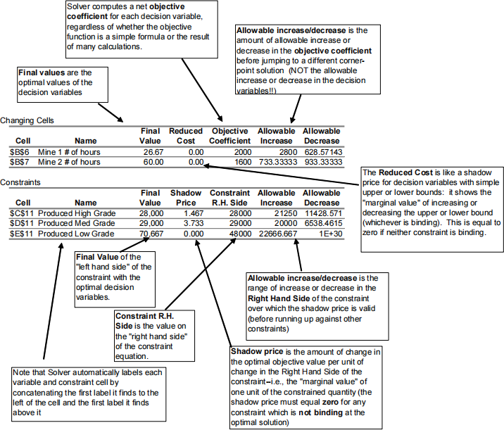
d) Interpreting Solver output and using the sensitivity report to determine consequences of relaxing constraints and/or changing objective coefficients. Remember, you can also always check the interpretation of a change by rerunning Solver. The annotated sensitivity report from Class 9 (copied on the next page) provides a good illustrative example of the meaning of each of these outputs. Make sure that you are familiar with each of these outputs and can use them to answer questions about the solution and the model. See the questions about the New Bedford problem for another good example of these sorts of questions.

e)  Using integer constraints where appropriate.