Hello, dear friend, you can consult us at any time if you have any questions, add WeChat: daixieit

MATH6173 Coursework 2

The coursework is due on 12-01-23 at 16.00. You should submit your work via Blackboard. You should submit a single RMarkdown or Quarto document that includes your code, descriptive answers to questions and generates any required plots. The document must compile on an independent computer. Please check your document carefully. A document that does not compile can receive at most 50% of the marks available.

You may use any function from base  R and  tidyverse . You may not use any other functions from other packages.

Marks will be awarded for accuracy of results and correctness of interpretation and discussion. Correctness of code is important, efficiency is not being assessed.

Ensure that all plots are informative and readable, including the use of appropriate plotting symbols/colours and axis labels.

Many of the questions rely on simulation and the generation of random numbers. You should use the  set.seed function to ensure that your results are reproducible. I suggest you use your student number as the seed, and set the seed once at the start of your document. Be sure to do a final check that any commentary you include agrees with the generated computational results.

Standard University rules for late work apply. All work must be carried out independently, and you are reminded of the University’s Academic Integrity Policy.

In the interests of fairness, queries which relate directly to the coursework must be made via the Discussion Forum on Blackboard. This ensures that  everybody has access to the same information.

The coursework is worth 50% of the module mark. There are four questions. Full marks can only be obtained if your code is free of errors.

Question 1 (10 marks)

Consider a random variable X with cumulative density function

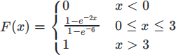
a.  Write a function that implements the inverse transformation method to generate random variables from this distribution. Compare graphically the empirical cumulative distribution function for 1000 samples with the true cumulative distribution function. Comment on the result.

b.  Use Monte Carlo integration to estimate E[cos(X)] using 1000 samples. Compare your result to the value obtained using a deterministic numerical integration method.

c.  Compute a 95% Monte Carlo confidence interval for E[cos(X)] using your results from part (b). Suppose we want the width of the confidence interval to be no more than 10−5. How many samples  would we need to achieve this? (As your answer should be a large number, write it in scientific notation for compactness.)

Question 2 (15 marks)

Assume a random variable X follows a Gamma distribution with density

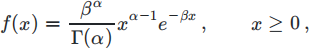
and shape parameter α = 3 and rate parameter β = 4. We are interesting in estimating the two integrals I1  = P (X > 2) and I2  = E [1/X].

a.  Estimate I1 and I2 using importance sampling with a standard normal importance density. Use 10000 samples. Compute a 95% confidence  interval for each estimate. Comment on the accuracy of your results.

b.  Suggest more appropriate importance densities for each of I1 and I2 . Justify your choices. Estimate I1 and I2 using importance sampling with these densities and 10000 samples. Compute a 95% confidence  interval for each estimate. Comment on the results.

Question 3 (15 marks)

Consider a random variable X with density

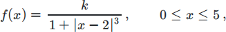
where k > 0 is a normalising constant.

a.  Write a function that implements a Metropolis algorithm to generate  from this density, using a normal proposal distribution centred at the current value of the chain and with standard deviation σ .

b.  Using σ = 5, estimate E(X 3 ) and P(X < 1) by running the algorithm for n = 5000 iterations. In each case, check your estimate by comparing to the result obtained by numerical integration.

c.  For σ = 0.05, run the algorithm four times for n = 5000 iterations, starting from x0  = 0, x0  = 1, x0  = 2 and x0  = 3. Compare the empirical cumulative distribution function for these four chains to a plot of the “true” distribution function, obtained using numerical integration. Comment on the results.

d.  Compare the algorithm for σ ∈ {0.05, 1, 5} in terms of the acceptance rate and of the resulting stationary distributions.

Question 4 (10 marks)