Hello, dear friend, you can consult us at any time if you have any questions, add WeChat: daixieit

Continuous Assessment 1

COMP528

In this assignment, you are asked to implement 2 algorithms for the Travelling Salesman Problem. This document explains the operations in detail, so you do not need previous knowledge. You are encouraged to start this as soon as possible. Historically, as the dead-line nears, the queue times on Barkla grow as more submissions are tested. You are also encouraged to use your spare time in the labs to receive help, and clarify any queries you have regarding the assignment.

1 The Travelling Salesman Problem (TSP)

The travelling salesman problem is a problem that seeks to answer the following question: ‘Given a list of vertices and the distances between each pair of vertices, what is the shortest possible route that visits each vertex exactly once and returns to the origin vertex?’.

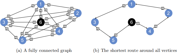
Figure 1: An example of the travelling salesman problem

The travelling salesman problem is an NP-hard problem, that meaning an exact solution cannot be solved in polynomial time. However, there are polynomial solutions that can be used which give an approximation of the shortest route between all vertices. In this assignment you are asked to implement 2 of these.

1.1 Terminology

We will call each point on the graph the vertex. There are 6 vertices in Figure 1.

We will call each connection between vertices the edge. There are 15 edges in Figure 1.z

We will call two vertices connected if they have an edge between them.

The sequence of vertices that are visited is called the tour. The tour for Figure 1(b) is (1, 3, 5, 6, 4, 2, 1). Note the tour always starts and ends at the origin vertex.

A partial tour is a tour that has not yet visited all the vertices.

2 The solutions

2.1 Preparation of Solution

You are given a number of coordinate files with this format:

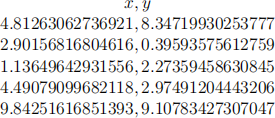
Figure 2: Format of a coord file

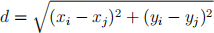
Each line is a coordinate for a vertex, with the x and y coordinate being separated by a comma. You will need to convert this into a distance matrix.

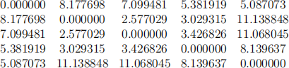
Figure 3: A distance matrix for Figure 2

To convert the coordinates to a distance matrix, you will need make use of the euclidean distance formula.

           (1)

Figure 4: The euclidean distance formula

Where: d is the distance between 2 vertices vi and vj , xi and yi are the coordinates of the vertex vi , and xj and yj are the coordinates of the vertex vj.

2.2 Cheapest Insertion

The cheapest insertion algorithm begins with two connected vertices in a partial tour. Each step, it looks for a vertex that hasn’t been visited, and inserts it between two connected vertices in the tour, such that the cost of inserting it between the two connected vertices is minimal.

These steps can be followed to implement the cheapest insertion algorithm. Assume that the indices i, j, k etc. are vertex labels, unless stated otherwise. In a tiebreak situation, always pick the lowest index or indices.

1. Start off with a vertex vi.

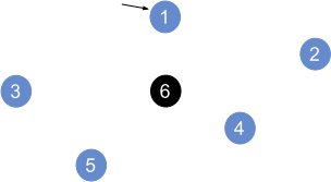
Figure 5: Step 1 of Cheapest Insertion

2. Find a vertex vj such that the dist(vi , vj ) is minimal, and create a partial tour (vi , vj , vi)

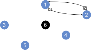
Figure 6: Step 2 of Cheapest Insertion

3. Find two connected vertices (vn, vn+1), where n is a position in the partial tour, and vk that has not been visited. Insert vk between vn and vn+1 such that dist(vn, vk) + dist(vn+1, vk) − dist(vn, vn+1) is minimal.

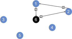
Figure 7: Step 3 of Cheapest Insertion

4. Repeat step 3 until all vertices have been visited, and are in the tour.

Figure 8: Step 4 of Cheapest Insertion

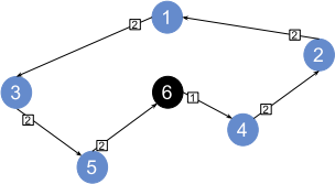
Figure 9: Final step and tour of Cheapest Insertion. Tour Cost = 11

2.3 Farthest Insertion

The farthest insertion algorithm begins with two connected vertices in a partial tour. Each step, it checks for the farthest vertex not visited from any vertex within the partial tour, and then inserts it between two connected vertices in the partial tour where the cost of inserting it between the two connected vertices is minimal.

These steps can be followed to implement the farthest insertion algorithm. Assume that the indices i, j, k etc. are vertex labels unless stated otherwise. In a tiebreak situation, always pick the lowest index(indices).

1. Start off with a vertex vi .

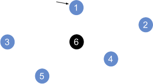
Figure 10: Step 1 of Farthest Insertion

2. Find a vertex vj such that dist(vi , vj ) is maximal, and create a partial tour (vi , vj , vi).

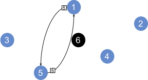
Figure 11: Step 2 of Farthest Insertion

3. For each vertex vn in the partial tour, where n is a position in the partial tour, find an unvisited vertex vk such that dist(vn, vk) is maximal.

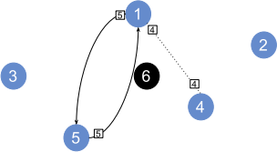
Figure 12: Step 3 of Farthest Insertion

4. Insert vk between two connected vertices in the partial tour vn and vn+1, where n is a position in the partial tour, such that dist(vn, vk) + dist(vn+1, vk) − dist(vn, vn+1) is minimal.

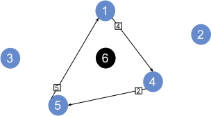
Figure 13: Step 4 of Farthest Insertion

5. Repeat steps 3 and 4 until all vertices have been visited, and are in the tour.

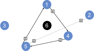
Figure 14: Step 3(2) of Farthest Insertion

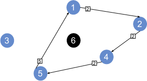
Figure 15: Step 4(2) of Farthest Insertion

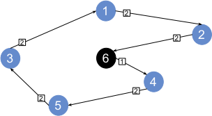
Figure 16: Final step and tour of Farthest Insertion. Tour Cost = 11

3 Running your programs

Your program should be able to be ran like so:

./<program   name>. exe  <coordinate   file   name > <output   file   name>

Therefore, your program should accept a coordinate file, and an output file as arguments. Note that C considers the first argument as the program executable.

Both implementations should read a coordinate file, run either cheapest insertion or farthest insertion, and write the tour to the output file.

3.1 Provided Code

You are provided with code that can read the coordinate input from a file, and write the final tour to a file. This is located in the file coordReader.c. You will need to include this file when compiling your programs.

The function readNumOfCoords() takes a filename as a parameter and returns the number of coordinates in the given file as an integer.

The function readCoords() takes the filename and the number of coordinates as parameters, and returns the coordinates from a file and stores it in a two-dimensional array of doubles, where coords[i ][0] is the x coordinate for the ith coordinate, and coords[i ][1] is the y coordinate for the ith coordinate.

The function writeTourToFile() takes the tour, the tour length, and the output filename as parameters, and writes the tour to the given file.

4 Instructions

• Implement a serial solution for the cheapest insertion and the farthest insertion. Name these: cInsertion.c, fInsertion.c.

• Implement a parallel solution, using OpenMP, for the cheapest insertion and the far-thest insertion. Name these: ompcInsertion.c, ompfInsertion.c.

• Create a Makefile and call it ”Makefile” which performs as the list states below. With-out the Makefile, your code will not grade on CodeGrade (see more in section 5.1).

– make ci compiles cInsertion.c and coordReader.c into ci.exe with the GNU com-piler

– make fi compiles fInsertion.c and coordReader.c into fi.exe with the GNU compiler

– make comp compiles ompcInsertion.c and coordReader.c into comp.exe with the GNU compiler

– make fomp compiles ompfInsertion.c and coordReader.c into fomp.exe with the GNU compiler

– make icomp compiles ompcInsertion.c and coordReader.c into icomp.exe with the Intel compiler

– make ifomp compiles ompfInsertion.c and coordReader.c into ifomp.exe the Intel compiler.

• Test each of your parallel solutions using 1, 2, 4, 8, 16, and 32 threads, recording the time it takes to solve each one. Record the start time after you read from the coordinates file, and the end time before you write to the output file. Do all testing with the large data file.

• Plot a speedup plot with the speedup on the y-axis and the number of threads on the x-axis for each parallel solution.

• Plot a parallel efficiency plot with parallel efficiency on the y-axis and the number of threads on the x-axis for each parallel solution.

• Write a report that, for each solution, using no more than 1 page per solution, describes: your serial version, and your parallelisation strategy

• In your report, include: the speedup and parallel efficiency plots, how you conducted each measurement and calculation to plot these, and sreenshots of you compiling and running your program. These do not contribute to the page limit

• Your final submission should be uploaded onto CodeGrade. The files you upload should be:

– Makefile

– cInsertion.c

– fInsertion.c

– ompcInsertion.c

– ompfInsertion.c

– report.pdf

5 Hints

You can also parallelise the conversion of the coordinates to the distance matrix.

When declaring arrays, it’s better to use dynamic memory allocation. You can do this by...

int ∗ o n e d a r ra y = ( int ∗) malloc ( numOfElements ∗ s i z e o f ( int ) ) ;

For a 2-D array:

int ∗∗ twod a r ra y = ( int ∗∗) malloc ( numOfElements ∗ s i z e o f ( int ∗ ) ) ;

for ( int i = 0 ; i < numOfElements ; i ++){

twod a r ra y [ i ] = ( int ∗) malloc ( numOfElements ∗ s i z e o f ( int ) ) ;

}

5.1 Makefile

You are instructed to use a MakeFile to compile the code in any way you like. An example of how to use a MakeFile can be used here:

{make command } : { t a r g e t f i l e s }

{compile command}

ci : cInsertion . c coordReader . c

gcc cInsertion . c coordReader . c −o c i . exe −lm

Now, in the Linux environment, in the same directory as your Makefile, if you type ‘make ci‘, the compile command is automatically executed. It is worth noting, the compile command must be indented. The target files are the files that must be present for the make command to execute.

6 Marking scheme

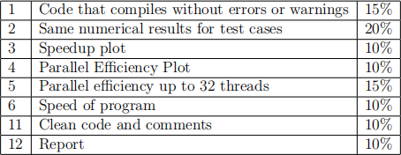
Table 1: Marking scheme

The purpose of this assessment is to develop your skills in analysing numerical programs and developing parallel programs using OpenMP. This assessment contributes to 40% of this modules grade. The scores from the above marking scheme will be scaled down to reflect that. Your work will be submitted to automatic plagiarism/collusion detection systems, and those exceeding a threshold will be reported to the Academic Integrity Officer for investigation regarding adhesion to the university’s policy https://www.liverpool.ac.uk/media/liva cuk/tqsd/code-of-practice-on-assessment/appendix_L_cop_assess.pdf.

7 Deadline

The deadline is the 17th November 2023

https://www.liverpool.ac.uk/aqsd/academic-codes-of-practice/code-of-practic e-on-assessment/