MATH6174: Likelihood and Bayesian Inference SEMESTER 1 EXAMINATION 2023/24
Hello, dear friend, you can consult us at any time if you have any questions, add WeChat: daixieit
SEMESTER 1 EXAMINATION 2023/24
MATH6174: Likelihood and Bayesian Inference
Duration: Due Date: January 12, 2024
1. [25 marks.] Suppose that we have a random sample of normal data
Yi ∼ N(μ, σ2 ), i = 1, . . . , n
where σ2 is known but μ is unknown. Thus for μ the likelihood function comes from the distribution
Y(¯) ∼ N(μ, σ2 /n),
where Y(¯) = ![]() :
:![]() Yi. Assume the prior distribution for μ is given by
Yi. Assume the prior distribution for μ is given by
N(出, σ2 /n0 ) where 出 and n0 are known constants.
(a) [10 marks] Show that the posterior distribution for μ is normal with
n0出 + n¯(g) σ 2
![]() mean = E(μ|¯(g)) =
mean = E(μ|¯(g)) = variance = var (μ|¯(g)) =
(b) [4 marks] Provide an interpretation for each of E(μ|¯(g)) and var(μ|¯(g)) in terms of the prior and data means and prior and data sample sizes.
(c) [4 marks] By writing a future observation Y(˜) = μ + E where E ∼ N(0, σ2 )
independently of the posterior distribution π(μ|¯(g)) explain why the posterior predictive distribution of Y(˜) given ¯(g) is normally distributed. Obtain the mean and variance of this posterior predictive distribution.
(d) [7 marks] Suppose that in an experiment n = 2, ¯(g) = 130, n0 = 0.25, 出 = 120 and σ2 = 25. Obtain:
(i) the posterior mean, E(μ|¯(g)) and variance, var(μ|¯(g)),
(ii) a 95% credible interval for μ given¯(g),
(iii) the mean and variance of the posterior predictive distribution of a future observation Y˜,
(iv) a 95% prediction interval for a future observation Y˜.
2. [25 marks.]
Suppose that y1 , . . . , yn are i.i.d. observations from a Poisson distribution with
mean θ where θ > 0 is unknown. Consider the following three models, that differ in the specification of the prior distribution of θ:
M1 : θ = 1,
M2 : π(θ) = ![]() θa−1 e −bθ, a > 0, b > 0, M3 : π(θ) ∝(I(θ),
θa−1 e −bθ, a > 0, b > 0, M3 : π(θ) ∝(I(θ),
where I(θ) is the Fisher information number (see the formula sheet for its definition).
(a) [8 marks] Write down the likelihood function. Hence obtain the Jeffreys prior for θ given by π(θ) =(I(θ).
(b) [10 marks] Derive an expression for the Bayes factor for comparing models M1 and M2 . If a = b = 1, n = 2 andy1 + y2 = 4, find the values of the
Bayes factor. Which model is preferred?
(c) [7 marks] Explain why it is problematic to use the Bayes factor to compare M3 with any of the other two models. Describe an alternative approach for comparing M3 with any other model and discuss how it can be implemented using Monte Carlo methods.
3. [25 marks.]
Assume that we want to use a Gibbs sampler to estimate P(X1 ≥ 0, X2 ≥ 0)
for a normal distribution N(µ, Σ), where µ = µ(µ)2(1) and Σ = σ12(σ12) σ22(σ12) .
The pdf of this distribution is
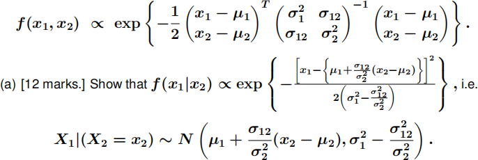
(b) [7 marks.] Write down the conditional distribution of X2 |(X1 = x1 )
(c) [6 marks.] Write down the steps for implementing the Gibbs sampler at some iteration t = 1, 2, . . .
4. [25 marks.] In the previous question consider the special case µ1 = µ2 = 0,
σ 1(2) = σ2(2) = 1 and σ12 = 0.4. Write (but do not include) the necessary code in R
to implement Gibbs sampler for this case (consider t = 1, 2, . . . , 4000 and
x![]() ∼ N(µ2 , σ2(2))).
∼ N(µ2 , σ2(2))).
(a) [5 marks.] Run the code to simulate 4000 samples from the joint distribution. Plot
the resulting chains and comment on the convergence behaviour of the chains.
(b) [5 marks.] Estimate E(X1 ), E(X2 ), Var(X1 ), Var(X2 ) and Corr(X1 , X2 ) along with their numerical standard errors. Compare your estimates with the
corresponding true values.
(c) [15 marks.] Estimate P(X1 ≥ 0, X2 ≥ 0). Using the resulting chains, calculate and plot the evolution of P(X1 ≥ 0, X2 ≥ 0) over time
t = 1, 2, . . . , 4000. Run the sampler 100 times and plot the replications of P(X1 ≥ 0, X2 ≥ 0) over time in grey (all in one plot). Add the original
estimate of P(X1 ≥ 0, X2 ≥ 0) as a black line over the plotted range. Hint: The required plot here is similar to the one shown in the lectures discussing Monte carlo estimation of π .
2023-12-27