Hello, dear friend, you can consult us at any time if you have any questions, add WeChat: daixieit

Department of Statistics

STATS 330: Advanced Statistical Modelling

Assignment 4

Semester 2, 2021

Notes:

(i) Write your assignment using R Markdown. Knit your report to either a Word or PDF document.

(ii) Create a section for each question. Include all relevant code and output in the final document.

(iii) Five presentation marks are available. Please think of your markers - keep your code and plots neat and remember to check your spelling. (R Markdown has an inbuilt spellchecker!)

(iv) Please remember to upload your Word or PDF document to CANVAS by the due date.

In this assignment, we will examine modelling from a number of perspectives — all of which should be considered when deciding how to model data:

● inspecting the data and making allowances for other background events pertinent to these data,

● looking at how these models fit your data,

● see how well the model predicts,

● using all the above ideas to see which model you are most comfortable with.

Question 1

In this question, we will revisit the caffeine data in Assignment 3 - Question 3 and and revisit it via the bootstrap re-sampling.

Caffeine peak data

Re-read the section describing these data from Assignment 3 - Question 3 — if necessary.

(a) Obtain 1000 non-parametric bootstrap estimates of xpeak from the data provided in Assignment 3 - Question 3 (referred to as Caffeine2.df). Plot a histogram of these estimates. Comment briefly.

[5 marks]

Note: You will need to obtain the original estimated xpeak calculated value from Assignment 3 - Question 3.

In order to do this non-parametrically, instead of using modeled probabilities, use the observed probabilities from your data.

An explanation by example —- the 0mg caffeine data point we observed y = 109 out of 300 trials. That is a grouping of a vector containing 109 1s and 191 0s . A random sample (with replacement) of 300 from a vector like this is the equivalent of random binomial sample

Y ∼ Binomial 

(b) Calculate a bootstrap confidence interval (CI) for xpeak based on these bootstrap samples.

[5 marks]

(c) How does this CI compare to the CI you obtained using simulation in Assignment 3 - Question 3.

[5 marks]

Question 2

The following example is based on a classic machine learning data set. The US post office wants to be able to electronically scan hand-written numbers and be able to predict what was written for the ZIP code. A ZIP code tells them where a mail item needs to be delivered. We will look at the numbers 3 and 7 only — to see if we can distinguish these two numbers — to illustrate ideas about prediction based on logistic regression.

In this assignment, you will be using logistic regression in the context of optical character recognition. Each line of the data set is a digital representation of a scanned hand-written digit, originally a part of a zip code handwritten on a US letter.

Each hand-written digit is represented as a 16 x 16 array of pixels, as in the examples below.

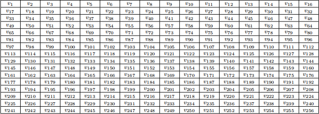
Each pixel is given a grey-scale value in the range [−1, 1] with -1 representing white and 1 representing black. There are thus 16 x 16 = 256 numbers representing a particular digit, which we can take as the values of 256 variables, v1, . . . , v256, say. The relationship between the pixels and the variables is as follows:

(a) Use the code below to import this training data. Make sure that there are no missing values, the variable D only has the values 3 and 7 and, that variables V1, V2 . . . V256 have values between −1 and 1.

[5 marks]

(b) The code below lets us look at the first 25 sample of handwritten 3s and 7s. Submit this code and comment of which of the 256 cells you think would be best at discrimination between a 3 and a 7. Comment briefly.

[5 marks]

In order to make the number of variables manageable we will get you to select the variables V1, V2 . . . V256 that have the highest correlation (in absolute terms - large negative or positive values) with the response variable D.

(c) Compute the correlation between D and V1, V2 . . . V256 and identify the which of these variables have the 20 highest absolute correlations (i.e. either large and negative or large and positive).

[5 marks]

Hints: The R functions names, sort and abs may be useful here.

(d) Fit a logistic model to the data, using the 20 variables you identified above. Call the model object Full.mod for future reference. (The regression will not converge if you use all 256 variables.)

Calculate the fitted logits for each of these hand-written digits.

[5 marks]

Hint: Append a binary variable Y to the data-frame train.df as follows:

(e) Use your fitted model to predict if a digit is a 3 or a 7 on the basis of the 20 variables. (Predict a digit to be a 7 if the fitted probability of a 7 is more than 0.5 (or equivalently, if the corresponding logit is positive.) Evaluate the in-sample prediction error (using the same data set to fit the model and evaluate the error).

[5 marks]

(f) Use the following code to do a step-wise variable selection process to choose a more parsimonious submodel of the 20-variable model. What are the in-sample prediction errors (PE) for this more parsimonious model and how does it compare to the PE for Full.mod calculated above?

[5 marks]

(g) Use cross-validation to estimate the prediction error rate (as a %) for this reduced model. Comment briefly.

Reminder: You will need to create a function called, say, PE.fun to do this.

[5 marks]

(h) Use the data set test.txt to calculate an estimate of the “out-of-sample” prediction error for the model used above. Here, we use the original data set to fit the model, and the new data to calculate the prediction error. Comment briefly on what this may indicate.

[5 marks]

(i) Challenge: Can you improve upon the prediction errors discussed above?

[Only glory! 0 marks]