Hello, dear friend, you can consult us at any time if you have any questions, add WeChat: daixieit

Department of Economics

ECON 351

Introductory Econometrics

Fall Term 2018/2019

Final Examination Make-Up

PART B: Short Answer Questions.

Answer all THREE of the following THREE questions. There is no choice in this section. Each part of each question is worth 5 marks.

Question B.1: Housing Prices (25 Marks)

You are interested in the the determinants of house prices, and have information on the log of the selling price of the house (lprice) number of bathrooms (baths), number of rooms (rooms), the age of the house (age), the squared age of the house (agesq), the natural log of the lot size (larea) as well as seven binary variables for the seven neighbourhoods in town (neighbourhoodi , i = 0,1,2,3,4,5,6). We run a regression with this data in Stata and get the following results:

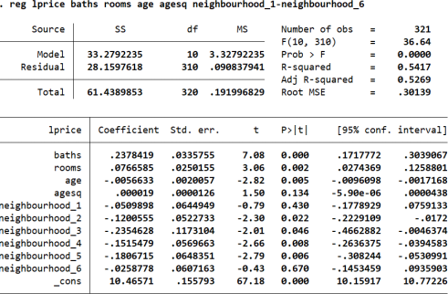
(a) Interpret the estimated coefficient on “neighbourhood 2”, as well as “rooms” .

(b) What is the marginal effect of age on the natural log of the selling price?  Draw a diagram of both the total and marginal effects of age on the natural log of the selling price of a house. Be sure to label important points. Does the relationship you find between selling price and age make sense?

(c) Explain how you would test whether what neighbourhood the house is in influences the selling price.  Clearly state your null and alternative hypothesis, explain how you calculate the test statistic, and explain how you draw a conclusion for your test.

(d) Your classmate suggests adding in an interaction term between the natural log of the size of the lot (larea) and the number of rooms in the the house.  Write out the regression with this interaction.  What is the marginal effect of adding a room to a house now? Interpret the theoretical coefficient on “rooms” in this new model, is it meaningful in this regression?

(e) Based on your model from (d), how would you directly estimate the average marginal effect of rooms on the natural log of housing price using a regression? How would you test that the average marginal effect is 0 with this new regression?

Question B.2: Loan Approval (25 Marks)

We are interested in the determinants of whether a person gets approved for a loan or not.  We have information on whether the loan was rejected, financial information and personal characteristics on a group of approx 2000 individuals who identify as either Hispanic, Black, or non-Black/non-Hispanic. We formulate the following model:

approve = α0 + α1 Black + α2 Hispanic + α3 atotinc + α4 Married + α5 Male + α6 obrat + u

where:

approve =  1 if the individual was approved for a loan (0 if rejected), atotinc is total monthly income, obrat measured other financial obligations as a percentage of total income.

We run regression we get the following results in Stata:

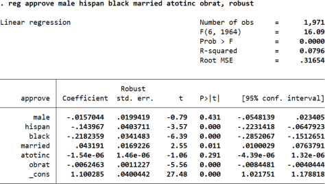
(a) What is the reference group here? Interpret the estimated coefficient on “Black”, and test whether it is significant at the 5% level.

(b) Why did we correct for heteroskedasticity here? Are there any other issues with linear probability models? Care- fully explain.

(c) Run a test of overall significance for this model.  Clearly state your null and alternative hypothesis, calculate the test statistic, and draw a conclusion for your test.

(d) Suppose we added interactions between “obrat” and Hispanic, as well as “obrat” and Black:

approve = α0 + α1 Black + α2 Hispanic + α3 atotinc + α4 Married

+ α5 Male + α6 obrat + α7 (obrat × Black) + α8 (obrat × Hispanic) + u

How would you interpret the α1  now? What about α7 ?

(e) What would happen to the coefficients and standard errors if we replaced the dependent variable with reject, which equals 1 if the person was rejected for the loan and 0 if not? Carefully explain.

Question B.3: School Voucher Program (15 Marks)