Read these instructions carefully:

• You are required to upload a PDF report as well as your code to Gradescope.

•  The report should be a maximum of 4 pages long with references included.  Minimum font size 10pts and margins of at least 1inch on A4 or standard letter size paper. You may use the template provided on Canvas.

•  Do not include your code in the pdf report and submit it separately to Gradescope.  Please upload the code as a single python script.

• Your report should be formatted as follows:

–  Title/author: Title of report, your name and email address. This is not meant to be a separate title page.

–  Sec.  1. Introduction and overview of the problem.

–  Sec. 2. Theoretical background and description of algorithms.

–  Sec. 3. Computational Results

–  Sec. 4.  Summary and Conclusions

–  References

•  I suggest you use LATEX(Overleaf is a great option) to prepare your reports.  A template is provided on Canvas under the Syllabus tab. You are also welcome to use Microsoft Word or any other software that properly typesets mathematical equations.

• I encourage collaborations, however, everything that is handed in (both your report and your code) should be your work.

• Your homework will be graded based on how completely you solved it as well as neatness and little things like: did you label your graphs and include figure captions. The homework is worth 10 points.  3 points will be given for the overall layout, correctness and neatness of the report, and 7 additional points will be for specific technical things and computational results that the TAs will look for in the report itself.

Problem Description

Your goal in this HW is to fit various types of models to a data set of fuel consumption (mpg) of various cars as a function of different attributes such as engine displacement, horsepower and weight. You will investigate the quality of your models and compare whether higher complexity results in better model performance.

•  Python users: Download the file mpg_train_test.npz from Canvas and load it using numpy.load.

•  MATLAB users:  Download the file mpg_train_test.mat from Canvas and load it using the load command.

•  The file auto-mpg.xls is also included which contains the raw data set. You do not need this file for the HW and it is only provided for those of you who are curious about it.

The provided files contain a training data set Xtrain , y train  where Xtrain  is a matrix of size 254 × 3 and y train is a vector of size 254.  The first column of Xtrain  contains engine displacements, second column contains horsepower, while the third column contains the curb weight of the vehicles.  The vector y train  contains the mpgs (fuel consumptions). The training data contains 254 instances. The test data set Xtest,y test  are analogous to the training data set but contain 138 instances.

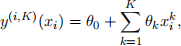
1.  Each data point in the training set has three features  (displacement,  horsepower, weight) which constitute the rows of the matrix Xtrain . We let x = (x1 , x2 , x3 ) ∈ R3  denote the set of features of a car and let y(x) ∈ R denote the mpg of that car. Your first task is to find a function y(x) that is only a function of one of the features.  More precisely consider functions of the form

(a)  (mpg as a function of displacement) y(1)(x1 ) =   0 +   1x1 +  2x1(2)

(b)  (mpg as a function of horsepower) y(2)(x2 ) =   0 +   1x2 +  2x2(2)

(c)  (mpg as a function of weight) y(3)(x3 ) =   0 +   1x3 +  2x3(2)

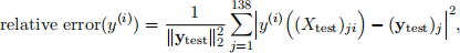
In other words, in each model you want to predict the mpg y as a function of one of the features only. For each of the above models formulate an appropriate least squares problem using the training data  set to find the parameters   j  that define the models (note, you will find a different    vector for each  model). In a table report the relative test error of each of your models

Also for each model present a 2D scatter plot of xi-vs-yi  of the test data overlaid with a line plot of your model y(i)(xi). Discuss your findings and report which feature is the better predictor of the mpg. Hint:  recall Vandermonde matrices.

2.  Now we consider higher order analogues of the models from part  1.  More precisely, consider K-th degree models of the form

for i = 1, 2, 3.  Repeat the experiments of part 1 by replacing the quadratic models in (a)–(c) with their  K-th degree counter parts for K = 4, 8, 12. Present a table containing the relative errors of each model  (9 models in total) and choice of K as well as the requisite scatter and line plots showing the behavior  of each model. Is there a point of diminishing returns in terms of the degree K?  Discuss your results. Hint 1: In your scatter plots you can plot each model y(i)  with three different values of K  on the same  plot to save space.  Don’t forget to generate a legend.

3.  Next we consider models that depend on multiple features at a time. Let